Decision Trees (A comprehensive Note)
Based on StatQuest with Josh Starmer: “Decision and Classification Trees, Clearly Explained!!!” and “Decision Trees, Part 2 — Feature Selection and Missing Data”, supplemented with additional theory and pointers.
Table of Contents
- What is a Decision Tree?
- Anatomy of a Tree
- How to Read a Decision Tree
- Building a Tree From Scratch
- Impurity Metrics
- Handling Continuous/Numeric Features
- Handling Categorical Features
- Feature Selection — Part 2 Content
- Handling Missing Data
- Overfitting and Pruning
- Regression Trees (Brief)
- Key Properties and Gotchas
- Practical Pointers (sklearn)
- Where Decision Trees Lead — the Bigger Picture
What is a Decision Tree?
A decision tree is a supervised learning algorithm that can handle both classification and regression. At its core it is just a flowchart of binary questions. You start at the top (the root) and follow true/false branches until you hit a terminal node (a leaf), which gives you a prediction.
Two flavours:
- Classification Tree — predicts a discrete class label (e.g., “will this patient get heart disease?”)
- Regression Tree — predicts a continuous value (e.g., “what drug dosage is optimal?”)
Josh Starmer’s analogy in StatQuest is perfect: a decision tree is literally how you’d explain a decision to a colleague step by step. That’s also why they’re used in high-stakes domains — medicine, finance, legal — where you need to justify a prediction, not just make it.
Anatomy of a Tree
              [Root Node]
             /            \
       True /              \ False
     [Internal Node]    [Internal Node]
       /        \             |
    [Leaf]    [Leaf]        [Leaf]
| Term | Meaning |
|---|---|
| Root Node | The very first split; the best single feature to start with |
| Internal Node (Branch) | An intermediate split based on some feature |
| Leaf Node (Terminal Node) | No further splits; contains the final prediction |
| Depth | Number of edges from root to a leaf |
| Pure Leaf | All samples in the leaf belong to the same class |
| Impure Leaf | Mixed classes; prediction is the majority class |
Convention (StatQuest): If a condition is true, you go left. If false, go right. Some libraries swap this — always check, but it doesn’t affect model quality.
How to Read a Decision Tree
Work top-down. At each node you’re answering a yes/no question about a feature. Keep following the branch matching your answer. When you reach a leaf, output the majority class (classification) or mean value (regression) of the training samples that fell into that leaf.
Example — Heart Disease Prediction:
Does the patient have chest pain?
     YES                        NO
      |                          |
Good blood                  Has the patient
circulation?               ever had a blockage?
  YES    NO                  YES         NO
   |      |                   |            |
Heart   Heart              Heart       No Heart
Disease Disease            Disease     Disease
 (impure) (leaf)           (leaf)      (leaf)
Even impure leaves are valid — the majority class wins. If 3/4 samples at a leaf have heart disease, the leaf predicts “heart disease” (with 75% confidence).
Building a Tree From Scratch
This is the core algorithm. The procedure is greedy and recursive:
Step 1 — Try every possible split
For every feature, try every possible threshold (for numeric) or every subset (for categorical) as a split candidate. This is $O(n \log n)$ per feature after sorting.
Step 2 — Score each split
Compute an impurity score for the resulting child nodes (more on this below).
Step 3 — Pick the best split
Choose the split that gives the greatest reduction in impurity (i.e., maximum information gain or Gini gain) or basically has the lowest impurity over the subspace of data for that particular decision pivot of the tree.
Step 4 — Recurse
Apply the same procedure to each child node. Stop when:
- A node becomes pure (only one class remains)
- You hit a max_depth limit
- A node has fewer samples than
min_samples_split - No split improves impurity
Full Example (StatQuest-style, heart disease dataset)
Data:
| Chest Pain | Good Circulation | Heart Disease |
|---|---|---|
| Yes | Yes | Yes |
| Yes | No | Yes |
| No | Yes | No |
| No | No | No |
| Yes | Yes | No |
To pick the root, compute Gini impurity for all possible categories and pick the minimum total weighted impurity.
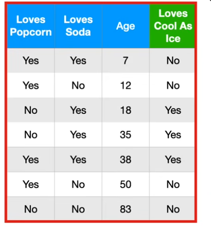 This is the example used in the StatQuest video. The green is the final decision we need to make with the other columns being features.
Impurity Metrics
Gini Impurity
Intuition: If you randomly pick a sample from a node and randomly assign it a class label (according to the class distribution at that node), what’s the probability you’d misclassify it?
$$\text{Gini}(t) = 1 - \sum_{i=1}^{C} p_i^2$$where $p_i$ is the fraction of samples at node $t$ belonging to class $i$, and $C$ is the number of classes.
Range: $[0, \frac{C-1}{C}]$. For binary classification: $[0, 0.5]$.
- 0 → perfectly pure node (all same class)
- 0.5 → maximum disorder (50/50 split)
Worked Example — Binary Node: Node has 4 samples: 3 “Yes”, 1 “No”
$$p_{\text{Yes}} = \frac{3}{4} = 0.75, \quad p_{\text{No}} = \frac{1}{4} = 0.25$$ $$\text{Gini} = 1 - (0.75^2 + 0.25^2) = 1 - (0.5625 + 0.0625) = 1 - 0.625 = 0.375$$For a split (weighted Gini): When you split a parent node into left and right children, compute the weighted average:
$$\text{Gini}_{\text{split}} = \frac{n_L}{n} \cdot \text{Gini}(L) + \frac{n_R}{n} \cdot \text{Gini}(R)$$where $n_L, n_R$ are sample counts in each child and $n = n_L + n_R$. The Gini Gain (information gain analog) is:
$$\Delta\text{Gini} = \text{Gini}(\text{parent}) - \text{Gini}_{\text{split}}$$You maximise $\Delta\text{Gini}$ (equivalently, minimise $\text{Gini}_{\text{split}}$) to choose the best split.
Numeric Feature Example:
Suppose you’re splitting on Age (sorted: 25, 30, 45, 52, 60). Candidate thresholds are the midpoints between consecutive values: 27.5, 37.5, 47.5, 56. For each threshold, partition the data, compute weighted Gini, pick the threshold with lowest weighted Gini as the representative of the split. (e.g below the age <15 is the representative of the age based split. although it was not used finally coz the other feature had lower gini impurity.)
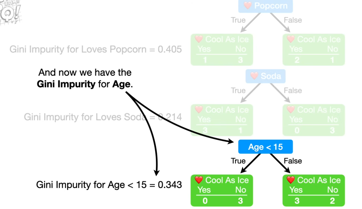 Since “Love Soda " has the lowest gini impurity we put it at the top of the tree.
Entropy and Information Gain
Intuition: Borrowed from information theory (Shannon entropy). Measures the average amount of information needed to describe the class of a sample.
$$H(t) = - \sum_{i=1}^{C} p_i \log_2(p_i)$$- 0 → pure node
- 1 → maximum disorder (binary case, 50/50 split)
Information Gain:
$$IG = H(\text{parent}) - \sum_{\text{children}} \frac{n_{\text{child}}}{n} \cdot H(\text{child})$$Same logic as Gini Gain — you pick the split maximising $IG$.
ID3 uses entropy + information gain. CART (sklearn’s implementation) uses Gini by default.
Gini vs Entropy
| Property | Gini Impurity | Entropy |
|---|---|---|
| Computation | Cheaper (no log) | Slightly more expensive |
| Range (binary) | [0, 0.5] | [0, 1] |
| Behavior | Tends to isolate the largest class | Slightly more exploratory |
| Used by | CART, sklearn (default), XGBoost | ID3, C4.5 |
| Practical difference | Usually negligible | Usually negligible |
Pointer: Don’t stress over Gini vs. Entropy — in practice they almost always produce the same tree. The performance difference is noise-level. Pick Gini if compute cost matters at scale.
Handling Continuous Features
This is important and StatQuest emphasises it. You can’t try every real number as a threshold — instead:
- Sort the feature values for the samples in the current node.
- Generate candidate thresholds = midpoints between consecutive distinct values.
- Evaluate each candidate’s weighted Gini (or IG).
- Keep the threshold with the lowest weighted Gini.
The same feature can be used multiple times in a tree at different nodes with different thresholds. This is perfectly valid and common.
Why midpoints? Any value between two consecutive sorted values gives the same split. The midpoint is conventional, clean, and numerically stable.
Handling Categorical Features
For a binary categorical feature (e.g., “has chest pain: Yes/No”), there’s only one possible split.
For a multi-valued categorical feature (e.g., colour: Red, Blue, Green), you can either:
- Try all binary partitions (e.g., {Red} vs {Blue, Green}, etc.) — exponential in the number of categories. CART does this for classification.
- One-hot encode and treat each category as a binary feature (common in sklearn).
Important nuance: C4.5 (unlike CART) uses Gain Ratio instead of raw information gain to penalise features with many distinct values, since a feature with a unique value per sample would perfectly split the tree on the training set but be useless for generalisation.
Feature Selection (Part 2 Content)
This is the content of the second video. It addresses what happens when a feature doesn’t cleanly improve things.
When a Feature Doesn’t Reduce Impurity
If no split on a particular feature reduces impurity (i.e., Gini Gain = 0 for all thresholds), that feature simply doesn’t get used at that node. The algorithm naturally performs implicit feature selection — you don’t need to do it manually.
Example: If “shoe size” doesn’t improve the Gini of predicting heart disease at any split point, it will never become a node in the tree.
Why the Same Feature Can Appear Multiple Times
A feature can appear at multiple levels in the tree with different thresholds. This is not overfitting by itself — it reflects the data’s actual decision boundaries.
Feature Importance (Side Note)
After training, you can compute feature importance as the total (weighted) Gini reduction a feature causes across all nodes where it’s used:
$$\text{Importance}(f) = \sum_{\text{nodes using } f} \frac{n_{\text{node}}}{n_{\text{total}}} \cdot \Delta\text{Gini}_{\text{node}}$$This is what clf.feature_importances_ gives you in sklearn.
Handling Missing Data
Also from Part 2. This is one of the most practically important topics.
Strategy 1: Imputation Before Splitting
Fill missing values with the most common value (categorical) or mean/median (numeric) in the training set before building the tree. Simple but can introduce bias.
Strategy 2: Surrogate Splits
During training, for each primary split, find a surrogate split — another feature that best mimics the behavior of the primary split. At inference, if the primary feature is missing, fall back to the surrogate. This is how CART natively handles it.
Strategy 3: Route to Both Branches
When a value is missing, send the sample down both branches, weighted by the proportion of training samples that went each way, then aggregate the leaf predictions. Used in XGBoost.
Strategy 4: Use Correlation
If feature A is missing but strongly correlated with feature B, use B’s value to estimate A. (This is essentially the surrogate split idea made explicit.)
Practical pointer: sklearn’s
DecisionTreeClassifierdoes not natively handle missing values (as of recent versions). You must impute beforehand usingSimpleImputeror similar. XGBoost/LightGBM handle missing data natively via the routing strategy.
Overfitting and Pruning
A decision tree that fully grows until every leaf is pure will memorise the training data — it will have near 100% training accuracy and poor test accuracy. This is the primary weakness of decision trees.
Why Trees Overfit
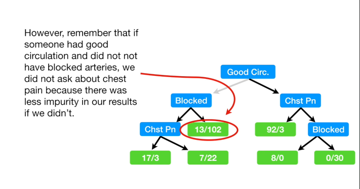
A fully grown tree creates arbitrarily complex, jagged decision boundaries that conform to every quirk and outlier in the training data. It models noise, not signal.
Pre-Pruning (Early Stopping)
Stop the tree from growing too big in the first place. sklearn hyperparameters:
| Parameter | What it does |
|---|---|
max_depth | Maximum tree depth. Most important knob. Start with 3–5. |
min_samples_split | Minimum samples required to split a node. Default: 2. Raise it. |
min_samples_leaf | Minimum samples required in a leaf. |
max_features | Number of features to consider per split (useful in ensembles). |
max_leaf_nodes | Cap the total number of leaves. |
Post-Pruning: Cost-Complexity Pruning (CCP)
Grow the full tree first, then prune backwards. This is the method highlighted in StatQuest’s follow-up videos and is the theoretically cleaner approach.
The Cost-Complexity Measure:
$$R_\alpha(T) = R(T) + \alpha \cdot |\tilde{T}|$$where:
- $R(T)$ = total impurity across all leaf nodes (training error proxy)
- $|\tilde{T}|$ = number of leaf nodes (model complexity)
- $\alpha \geq 0$ = regularisation strength (the “complexity parameter”)
Interpretation:
- $\alpha = 0$ → full unpruned tree (no complexity penalty)
- Higher $\alpha$ → aggressively removes branches (penalises large trees)
- For each $\alpha$, there’s an optimal subtree. You sweep over $\alpha$ values using cross-validation to pick the one with best test accuracy.
In sklearn:
from sklearn.tree import DecisionTreeClassifier

# Get pruning path
clf = DecisionTreeClassifier()
path = clf.cost_complexity_pruning_path(X_train, y_train)
ccp_alphas = path.ccp_alphas  # sequence of alphas

# Train a tree for each alpha
clfs = []
for alpha in ccp_alphas:
    clf = DecisionTreeClassifier(ccp_alpha=alpha)
    clf.fit(X_train, y_train)
    clfs.append(clf)

# Pick the alpha that maximises validation accuracy
Rule of thumb: Start with max_depth=3 or max_depth=5 before worrying about CCP. CCP is better in theory but adds engineering overhead.
Regression Trees
The procedure is essentially the same, but instead of Gini/Entropy you minimise variance (or mean squared error) within each child node.
$$\text{SSR} = \sum_{i \in \text{leaf}} (y_i - \bar{y}_{\text{leaf}})^2$$The best split is the one that minimises the total weighted SSR across children. Leaf predictions are the mean of the target values at that leaf.
Key difference from classification trees: You’re no longer looking for purity — you’re looking for low variance within each partition.
Regression trees are the building blocks of Gradient Boosting (XGBoost, LightGBM). Each boosting round fits a shallow regression tree to the residuals of the previous prediction.
Key Properties and Gotchas
Strengths
- Interpretable — literally a flowchart. Easy to explain to non-technical stakeholders.
- No feature scaling needed — splits are threshold comparisons, not distance-based.
- Handles mixed data types — numeric and categorical features together, natively.
- Non-parametric — no assumptions about data distribution.
- Implicit feature selection — irrelevant features simply never get split on.
Weaknesses
- High variance — small changes in training data can produce entirely different trees. This is why they’re usually used inside ensembles (Random Forests, Gradient Boosting).
- Greedy — each split is locally optimal, not globally optimal. The globally optimal tree is NP-complete to find; CART uses a greedy heuristic.
- Axis-aligned splits only — standard trees can only split parallel to feature axes. Diagonal decision boundaries require many splits. (Oblique trees exist but aren’t common.)
- Poor extrapolation — a regression tree can only predict values in the range of training targets. It can’t extrapolate beyond observed ranges.
- Piecewise constant output — predictions are not smooth. Regression trees produce step functions.
Common Mistakes
- Not pruning — running
DecisionTreeClassifier()with default settings is almost always going to overfit. Always tunemax_depthat minimum. - Forgetting that feature importance can be misleading — high-cardinality features (many unique values) tend to get spuriously high importance because there are more possible thresholds.
- Treating feature importance as global — SHAP values give more reliable local explanations.
Practical Pointers (sklearn)
from sklearn.tree import DecisionTreeClassifier, plot_tree
from sklearn.model_selection import cross_val_score
import matplotlib.pyplot as plt

# Basic fit
clf = DecisionTreeClassifier(
    criterion='gini',       # or 'entropy'
    max_depth=5,            # start here
    min_samples_leaf=5,     # prevents tiny, noisy leaves
    random_state=42
)
clf.fit(X_train, y_train)

# Visualise
fig, ax = plt.subplots(figsize=(20, 10))
plot_tree(clf, feature_names=feature_names, class_names=class_names,
          filled=True, ax=ax)
plt.show()

# Cross-validated accuracy
scores = cross_val_score(clf, X, y, cv=5)
print(f"Accuracy: {scores.mean():.3f} ± {scores.std():.3f}")

# Feature importances
importances = clf.feature_importances_
Hyperparameter tuning order of priority:
max_depth— most impactfulmin_samples_leaf— second most impactfulccp_alpha— if you want post-pruningcriterion— almost never matters
Where Decision Trees Lead — the Bigger Picture
Understanding decision trees deeply matters because they’re the base for almost every major tabular ML method:
| Method | How Trees Are Used |
|---|---|
| Random Forest | Averages predictions of many decorrelated trees trained on bootstrap samples. Fixes high variance. |
| Gradient Boosting (XGBoost, LightGBM, CatBoost) | Sequentially fits shallow regression trees to residuals. Fixes bias. |
| AdaBoost | Sequentially trains stumps (depth-1 trees), reweighting misclassified samples. |
| Isolation Forest | Uses random trees to isolate anomalies — outliers are isolated with fewer splits. |
The intuition you build from one tree — splits, impurity, leaves, overfitting — transfers directly to all of these.
Quick Reference Cheatsheet
BUILDING A TREE
1. Try every feature × every threshold as a split
2. For each split: compute weighted Gini of children
3. Pick the split with lowest weighted Gini
4. Recurse on each child node
5. Stop when: pure leaf | max_depth hit | too few samples

GINI IMPURITY
Gini(t) = 1 - Σ pᵢ²
Range [0, 0.5] for binary. 0 = pure, 0.5 = max disorder.

INFORMATION GAIN
IG = H(parent) - Σ (nᵢ/n) * H(child_i)
H(t) = -Σ pᵢ log₂(pᵢ)

STOPPING THE OVERFIT
max_depth=3-5  |  min_samples_leaf=5-20  |  ccp_alpha (tune via CV)

MISSING DATA
sklearn: impute first
XGBoost/LightGBM: handle natively (route to better branch)

KEY INTUITIONS
- Trees are greedy (locally optimal splits, not globally)
- Same feature can appear multiple times with different thresholds
- Irrelevant features are implicitly ignored
- Leaves predict majority class (classification) or mean (regression)
- Purity ≠ correctness; a pure leaf can still be wrong on new data
Sources: StatQuest “Decision and Classification Trees, Clearly Explained!!!” (2021), StatQuest “Decision Trees Part 2 — Feature Selection and Missing Data” (2018), sklearn documentation on Decision Trees and Cost Complexity Pruning.