Singular Value Decomposition(SVD)
A decomposition that reveals the skeleton of any matrix — no matter how complex.
1. The Core Idea
Every matrix $A$ (even non-square ones) can be factored into three matrices:
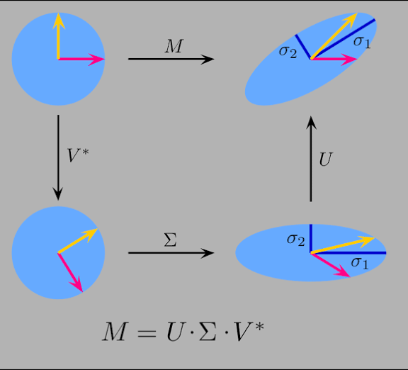
$$A = U \Sigma V^T$$Think of it this way: any linear transformation can be broken into three simple steps:
- Rotate the input space (via $V^T$)
- Scale along each axis (via $\Sigma$)
- Rotate again in the output space (via $U$)
That’s it. Any matrix — no matter how messy — is just rotate → stretch → rotate.
2. The Three Matrices
Given an $m \times n$ matrix $A$:
$U$ — Left Singular Vectors ($m \times m$)
- Columns are called left singular vectors
- They span the output space (column space of $A$)
- $U$ is orthogonal: $U^T U = I$
- Think: “the output directions”
$\Sigma$ — Singular Values ($m \times n$ diagonal)
- Diagonal entries $\sigma_1 \geq \sigma_2 \geq \cdots \geq \sigma_r \geq 0$ are the singular values
- They measure how much each direction is stretched
- $r = \text{rank}(A)$ non-zero singular values
- Think: “the importance scores”
$V^T$ — Right Singular Vectors ($n \times n$)
- Rows of $V^T$ (= columns of $V$) are called right singular vectors
- They span the input space (row space of $A$)
- $V$ is orthogonal: $V^T V = I$
- Think: “the input directions”
3. A Small Example
Take a $3 \times 2$ matrix representing, say, three documents and two topics:
$$A = \begin{bmatrix} 1 & 2 \\ 3 & 1 \\ 2 & 3 \end{bmatrix}$$SVD gives us:
- $U$ ($3 \times 3$): how each document relates to each latent axis
- $\Sigma$ ($3 \times 2$): how important each latent axis is (larger $\sigma$ = more important)
- $V^T$ ($2 \times 2$): how each topic relates to each latent axis
The first column of $U$ and first row of $V^T$, scaled by $\sigma_1$, give the single best rank-1 approximation of $A$.
4. The Rank-k Approximation — The Key Insight
SVD allows you to write any matrix as a sum of rank-1 matrices:
$$A = \sigma_1 u_1 v_1^T + \sigma_2 u_2 v_2^T + \cdots + \sigma_r u_r v_r^T$$Each term $\sigma_i u_i v_i^T$ is an outer product — a rank-1 matrix. They’re sorted by importance: $\sigma_1$ is the biggest, so the first term captures the most structure.
Truncated SVD (rank-$k$ approximation):
$$A_k = \sum_{i=1}^{k} \sigma_i u_i v_i^T$$This is the best possible rank-$k$ approximation of $A$ in terms of Frobenius norm. No other rank-$k$ matrix is closer to $A$. (This is the Eckart–Young–Mirsky theorem.)
What this means: you can compress information by keeping only the top $k$ singular triplets, discarding the rest. The singular values tell you exactly how much you’re losing.
5. Connection to Eigendecomposition
SVD and eigendecomposition are closely related:
- The columns of $U$ are eigenvectors of $AA^T$
- The columns of $V$ are eigenvectors of $A^T A$
- The singular values $\sigma_i = \sqrt{\lambda_i}$ where $\lambda_i$ are the eigenvalues of $A^T A$
For symmetric positive semi-definite matrices (like covariance matrices), SVD and eigendecomposition coincide. This is why PCA works.
6. Geometric Intuition
Imagine $A$ as a transformation of the unit sphere in $\mathbb{R}^n$:
- $V^T$ rotates the sphere (no distortion)
- $\Sigma$ stretches each axis: axis $i$ gets scaled by $\sigma_i$, turning the sphere into an ellipsoid
- $U$ rotates the ellipsoid into the output space
The semi-axis lengths of the resulting ellipsoid are exactly the singular values $\sigma_1, \sigma_2, \ldots$. Large $\sigma_i$ = fat axis = lots of variance in that direction. Small $\sigma_i$ ≈ 0 = the matrix is nearly rank-deficient in that direction.
7. Key Properties
| Property | What it means |
|---|---|
| Always exists | Every real matrix has an SVD, even non-square ones |
| Singular values ≥ 0 | Always real and non-negative, even for complex $A$ |
| $\text{rank}(A)$ = number of non-zero $\sigma_i$ | Rank is directly readable from SVD |
| $\|A\|_2 = \sigma_1$ | The spectral norm equals the largest singular value |
| $\|A\|_F = \sqrt{\sum \sigma_i^2}$ | Frobenius norm from singular values |
| Condition number = $\sigma_1 / \sigma_r$ | Large ratio → ill-conditioned system |
| $\det(A) = \prod \sigma_i$ (square $A$) | Determinant from singular values |
8. SVD vs PCA — Clearing Up the Confusion
People conflate SVD and PCA constantly. Here’s the precise relationship:
PCA finds the directions of maximum variance in data. Given a centered data matrix $X$ ($n$ samples, $d$ features):
- Compute the covariance matrix: $C = \frac{1}{n-1} X^T X$
- Eigendecompose: $C = V \Lambda V^T$
But notice: $X^T X \propto C$, and SVD of $X$ gives $X = U \Sigma V^T$, so:
$$X^T X = V \Sigma^2 V^T$$The columns of $V$ from SVD of $X$ are the PCA directions (principal components). The singular values relate to explained variance: $\text{Var}_i \propto \sigma_i^2$.
So PCA is SVD applied to the centered data matrix. Numerically, computing SVD of $X$ directly is more stable than computing the covariance matrix first (avoids squaring condition numbers).
9. Applications in Machine Learning
9.1 Dimensionality Reduction (PCA / Truncated SVD)
The most direct use. Keep the top $k$ singular vectors and project data into a lower-dimensional space:
$$X_{\text{reduced}} = X V_k$$where $V_k$ contains only the first $k$ columns of $V$.
- When $X$ is dense: Use PCA (center first, then SVD)
- When $X$ is sparse (e.g., TF-IDF matrices): Use TruncatedSVD directly (no centering — centering destroys sparsity). This is also called Latent Semantic Analysis (LSA) in NLP.
The scree plot of $\sigma_i^2$ (or explained variance ratio) tells you how many components to keep.
9.2 Recommender Systems (Matrix Factorization)
This is where SVD became famous in ML via the Netflix Prize.
Given a user-item rating matrix $R$ (mostly missing entries):
$$R \approx U \Sigma V^T$$- Rows of $U$: user embeddings in latent factor space
- Rows of $V$: item embeddings in latent factor space
- $\sigma_i$: importance of latent factor $i$
To predict user $u$’s rating for item $i$: take the dot product of their latent vectors.
In practice, you use SVD++ or ALS (Alternating Least Squares) since classic SVD doesn’t handle missing values. But the intuition is pure SVD: find the latent factors that best reconstruct observed ratings.
9.3 Natural Language Processing — LSA and Word Embeddings
Latent Semantic Analysis (LSA):
Build a term-document matrix $T$ where $T_{ij}$ = TF-IDF of term $i$ in document $j$. Apply SVD:
$$T \approx U_k \Sigma_k V_k^T$$- Rows of $U_k$: dense word vectors (each word gets a $k$-dim embedding)
- Rows of $V_k$: dense document vectors
- Words with similar meaning end up close in the latent space
This is a precursor to Word2Vec and BERT — same idea, different optimization.
Connection to modern embeddings: Word2Vec’s skip-gram with negative sampling has been shown to implicitly factorize a shifted PMI matrix — which is SVD in disguise. SVD embeddings and neural embeddings are more related than they look.
9.4 Low-Rank Adaptation (LoRA) — Fine-tuning Large Models
This is extremely relevant to modern LLMs. The insight: the update to a pre-trained weight matrix $W$ during fine-tuning tends to be low-rank.
LoRA parameterizes the update as:
$$\Delta W = AB \quad \text{where } A \in \mathbb{R}^{m \times r},\ B \in \mathbb{R}^{r \times n},\ r \ll \min(m,n)$$This is exactly a rank-$r$ factorization — the same structure SVD reveals. Instead of fine-tuning all $mn$ parameters of $W$, you fine-tune only $r(m + n)$ parameters.
Why does this work? Because the “important” weight updates lie in a low-rank subspace. SVD is the theoretical justification for why this approximation is reasonable.
9.5 Solving Linear Systems and Least Squares
For an overdetermined system $Ax \approx b$ (more equations than unknowns), the least-squares solution is:
$$x^* = A^+ b = V \Sigma^+ U^T b$$where $A^+$ is the Moore-Penrose pseudoinverse and $\Sigma^+$ replaces each non-zero $\sigma_i$ with $1/\sigma_i$.
This is numerically the most stable way to solve least squares — used under the hood by np.linalg.lstsq, scikit-learn’s LinearRegression, and many others.
Regularization connection: Ridge regression (L2) modifies the pseudoinverse:
$$x^*_\lambda = V \text{diag}\!\left(\frac{\sigma_i}{\sigma_i^2 + \lambda}\right) U^T b$$Small singular values get more heavily shrunk. SVD makes the geometry of regularization transparent.
9.6 Data Compression and Denoising
Image compression: An image is a matrix of pixel intensities. Keep only the top $k$ singular triplets:
- Original: $m \times n$ values
- Compressed: $k(m + n + 1)$ values
As $k$ increases, the reconstruction improves. The removed components often correspond to noise.
Denoising: If $A = A_{\text{signal}} + \text{noise}$, the noise tends to spread across all singular values while the signal concentrates in the top ones. Truncating at rank $k$ effectively filters noise. This is the basis of methods like randomized SVD for large-scale denoising.
9.7 Continual Learning — Subspace Perspective
This is a less-known but theoretically rich connection. When a neural network is trained on task $T_1$ and then task $T_2$, forgetting occurs because updates to $W$ overwrite the directions needed for $T_1$.
SVD provides a natural language for this:
- The column space of the gradient for $T_2$ reveals which directions in weight space are being updated
- If you project the $T_2$ gradient orthogonal to the row space of previously seen gradients (computed via SVD of a gradient matrix), you can update without interfering
This is the idea behind Gradient Projection Memory (GPM) and related CL methods. The singular vectors of past gradient matrices define the “protected subspace” for previously learned knowledge.
9.8 Neural Network Analysis
SVD is used to analyze and compress trained networks:
- Singular value spectrum of weight matrices: In well-trained networks, weight matrices often show a heavy-tailed singular value distribution. Random/untrained matrices have flat spectra. This has been used as a measure of model quality without access to data.
- Weight matrix compression: Replace a large weight matrix $W \approx U_k \Sigma_k V_k^T$ with two smaller matrices $A = U_k \Sigma_k^{1/2}$ and $B = \Sigma_k^{1/2} V_k^T$. Reduces parameters for inference.
- Intrinsic dimensionality: The effective rank of activations (number of significant singular values) measures how much of the model’s capacity is being used — relevant to over-parameterization and capacity questions in CL.
10. Computational Aspects
Full SVD
Exact SVD of an $m \times n$ matrix costs $O(\min(m,n) \cdot mn)$ — expensive for large matrices.
Truncated SVD
When you only need the top $k$ components, use iterative methods (Lanczos, ARPACK). Cost: $O(mnk)$, much cheaper for small $k$.
In practice: scipy.sparse.linalg.svds or sklearn.decomposition.TruncatedSVD.
Randomized SVD
For very large matrices, randomized SVD (Halko et al., 2011) gives approximate top-$k$ SVD in $O(mn \log k)$ with high probability. Used in scikit-learn’s TruncatedSVD for large sparse matrices.
When to Use What
| Scenario | Method |
|---|---|
| Small/medium dense matrix, full SVD needed | np.linalg.svd |
| Large dense, top-$k$ only | Randomized SVD (sklearn) |
| Large sparse, top-$k$ only | scipy.sparse.linalg.svds |
| Streaming / online updates | Incremental SVD (Brand 2002) |
11. Quick Reference
import numpy as np
from sklearn.decomposition import TruncatedSVD

# Full SVD (numpy)
U, S, Vt = np.linalg.svd(A, full_matrices=False)
# Rank-k approximation
A_k = U[:, :k] @ np.diag(S[:k]) @ Vt[:k, :]

# Truncated SVD for large/sparse matrices (sklearn)
svd = TruncatedSVD(n_components=k)
X_reduced = svd.fit_transform(X)  # shape: (n_samples, k)
# Explained variance
print(svd.explained_variance_ratio_.cumsum())

# Pseudoinverse
A_pinv = np.linalg.pinv(A)  # uses SVD internally
12. Summary
| Concept | One-liner |
|---|---|
| What SVD does | Decomposes any matrix into rotate → scale → rotate |
| The singular values | Measure importance of each latent direction |
| Rank-$k$ approximation | Best possible low-rank summary of a matrix |
| PCA | SVD on the centered data matrix |
| LSA | SVD on the term-document matrix |
| LoRA | Fine-tuning via low-rank updates justified by SVD |
| Pseudoinverse | Stable solution to least squares via SVD |
| CL / Subspace methods | SVD defines “protected directions” for avoiding forgetting |
The singular value decomposition is one of those tools where once you understand it, you start seeing it everywhere in ML — in the theory, in the algorithms, and in the geometry of what your models are actually doing.