Definition

α is a threshold you fix in advance, before seeing any data. It’s the maximum probability of a Type I error (false positive — rejecting H₀ when H₀ is actually true) that you’re willing to tolerate.

Formally, if you reject H₀ when your data falls in some rejection region $R$, then a level-α test requires:

$$\sup_{\theta \in \Theta_0} P_\theta\big((X_1,\ldots,X_n) \in R\big) \leq \alpha$$

In words: no matter which specific θ in the null region $\Theta_0$ happens to be true, the chance your test wrongly rejects H₀ is at most α.

Use

α is the design parameter for your test — you pick it first, then build (or solve for) a rejection region $R$ (or equivalently a cutoff $c$) that satisfies the constraint above.

Common choices: α = 0.05, α = 0.01, α = 0.10. Once α is fixed:

• You compute your test statistic from data.
• You reject H₀ if the statistic falls in the rejection region tied to that α (equivalently, if p-value < α).
• The decision is binary: reject or don’t reject — nothing in between.

This is why α is often called the significance level: it’s the standard of proof you commit to before looking at the evidence, so you can’t move the goalposts after seeing the result.

Intuition

Think of α like a tolerance for wrongly crying wolf.

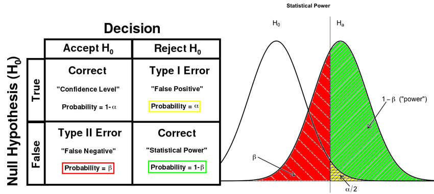
• If H₀ is actually true (there’s really no effect, the coin really is fair, etc.), α tells you how often you’re okay with your test mistakenly claiming there is something going on.
• α = 0.05 means: “If I ran this exact experiment many times under a true null, I’m okay with false alarms happening about 5% of the time.”

Courtroom analogy: α is like how strict the burden of proof is for a conviction. A smaller α (like 0.01) is a stricter court and so it is harder to convict someone of being guilty => fewer innocent people wrongly convicted. But this also means that some guilty ones walk free (lower power). A larger α (like 0.10) is a more lenient court, it is easier to convict, but more risk of convicting the innocent. (in the above figure, consider left side as innocent and right side as guilty )

---

The Main Tradeoff for $\alpha$

The key insight: R is one fixed region, used for both cases

Here’s the subtlety you’re circling: there’s only one rejection region $R$ (or one cutoff $c$). You don’t get a different $R$ depending on whether H₀ or H₁ is secretly true — you build $R$ once, then whatever the true θ actually is, the same $R$ decides your action.

So when you shrink α, you’re not shrinking “the false positive region” while leaving everything else untouched — you’re shrinking $R$ itself. And since $R$ is the same region used to detect real effects too, shrinking it necessarily makes it harder to land in $R$ even when H₁ is true.

Concrete example: coin flip

Say you flip a coin 100 times, testing “fair coin” (H₀) vs “biased coin” (H₁). Your rejection region is “reject if heads count is very extreme.”

• α = 0.10 (lenient): reject if heads < 40 or heads > 60. Wide region — easy to land in.
• α = 0.01 (strict): reject if heads < 32 or heads > 68. Narrow region — hard to land in.

Now suppose the coin actually is biased (H₁ true), say P(heads) = 0.58. With the lenient region, a heads-count around 58 easily clears the >56… sorry — clears the >60 line often enough. With the strict region, you need heads > 68, which a mildly-biased coin will hit much less often.

Same biased coin, same effect size — but the stricter α gives you way less chance of actually catching it.

So yes — your conclusion is correct

$$\alpha \downarrow \quad \Rightarrow \quad R \text{ shrinks} \quad \Rightarrow \quad \beta(\theta) \text{ decreases for } \theta \in \Theta_1 \text{ too} \quad \Rightarrow \quad \text{power} \downarrow \quad \Rightarrow \quad \text{Type II error (false negative)} \uparrow$$

This is exactly the tradeoff. Type I error and Type II error pull in opposite directions for a fixed sample size and fixed test statistic. You cannot shrink both simultaneously just by moving the cutoff $c$ — moving $c$ to help one always hurts the other.

The only way to escape the tradeoff

The one lever that can reduce both errors simultaneously is increasing your sample size $n$. More data sharpens your test statistic’s distribution (tighter concentration around the true θ), so you can push $c$ to reduce α without proportionally sacrificing power. This is really the whole motivation behind power analysis and sample size calculations in study design.

One-line takeaway: α and power move in opposite directions when you slide the cutoff — the only way to lower Type I error without paying for it in Type II error is to collect more data.

Want me to add this tradeoff explanation into the alpha note as an addendum?