Parent: Probability and Statistics

Power is β(θ) evaluated at a specific θ in Θ₁

Recall the power function:

$$\beta(\theta) = P_\theta\big((X_1,\ldots,X_n) \in R\big)$$

This is defined for every θ, but it means different things depending on which region θ sits in:

• When $\theta \in \Theta_0$: $\beta(\theta)$ = probability of a false positive at that θ. You want this small (≤ α).
• When $\theta \in \Theta_1$: $\beta(\theta)$ = probability of correctly rejecting H₀ — this is the power at that θ.

So “power” isn’t a single number in general — it’s a function of θ, because how easy it is to detect an effect depends on how far that particular θ is from H₀. A coin biased at P(heads)=0.9 is way easier to detect than one biased at P(heads)=0.51. That’s why you’ll often see “power at θ = ___” rather than just “the power.”

Worked example: normal mean test

Setup: $X_1,\ldots,X_n \sim N(\theta, 1)$, testing $H_0: \theta = \theta_0$ vs $H_1: \theta \neq \theta_0$, rejecting when $|T_n| > c$ where $T_n = \sqrt{n}(\bar X_n - \theta_0)$.

Step 1 — find c from α. Under $H_0$, $T_n \sim N(0,1)$, so you pick $c = z_{\alpha/2}$ (the standard normal critical value, e.g. 1.96 for α = 0.05).

Step 2 — ask: what if the true mean is actually some $\theta_1 \neq \theta_0$? Under this true θ₁, $T_n$ is no longer standard normal — it’s shifted:

$$T_n = \sqrt{n}(\bar X_n - \theta_0) \sim N\big(\sqrt{n}(\theta_1 - \theta_0),\ 1\big)$$

Why? Because $\bar X_n \sim N(\theta_1, 1/n)$ when θ₁ is the true mean, so $\sqrt n(\bar X_n - \theta_0)$ has mean $\sqrt n (\theta_1-\theta_0)$ and variance 1. Call this shift $\delta = \sqrt{n}(\theta_1 - \theta_0)$ — it’s essentially “the true effect size, scaled up by sample size.”

Step 3 — compute the power directly.

$$\text{Power}(\theta_1) = P_{\theta_1}(|T_n| > c) = P(|Z + \delta| > c)$$

where $Z \sim N(0,1)$. Expanding this out:

$$\text{Power}(\theta_1) = 1 - \Phi(c - \delta) + \Phi(-c-\delta)$$

That messy-looking expression is just: “the probability the shifted normal curve still lands past your cutoff $c$ in either tail.”

---

The intuition, stripped of formulas

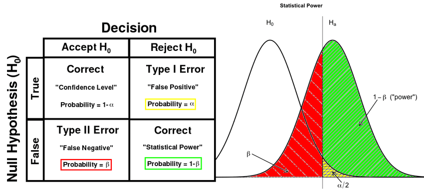Picture two bell curves on the same axis:

• Your rejection region is “past the cutoff $c$” (shaded tail).
• Power = how much of the H₁ curve’s area falls in that shaded rejection zone.

This picture makes every dependency obvious:

• Bigger effect size (θ₁ far from θ₀, so δ is large) → H₁ curve shifts far away from H₀ curve → more of it clears the cutoff → higher power.
• Smaller α → cutoff $c$ moves further out → less area under H₁ curve clears it → lower power (this is the α/power tradeoff).
• Bigger sample size $n$ → δ = √n(θ₁−θ₀) grows, and the curves get narrower (variance shrinks) → separation between the two curves increases faster than the cutoff moves → higher power without needing to loosen α. This is why more data breaks the tradeoff.

In practice (how it’s actually calculated)

For power analysis in real study design:

1. Pick α (e.g. 0.05) → gives you $c$.
2. Pick a minimum effect size you care about detecting (this is θ₁ − θ₀, or δ) — this is a judgment call, not derived from data.
3. Plug into the power formula above (or software like power.t.test in R, or statsmodels.stats.power in Python) to get a number like “80% power.”
4. Often flipped around: fix your desired power (commonly 80%) and solve for the sample size $n$ needed to hit it — this is the standard “sample size calculation” you see in papers.

One-line takeaway: power is the area of the H₁-true sampling distribution that falls inside your rejection region — driven by effect size, sample size, and how strict α forces the cutoff to be.