#compvis #interpretebility #ood-generalisation #robust-learning #to-ponder

Paper- \[2603.25839\] A Compression Perspective on Simplicity Bias

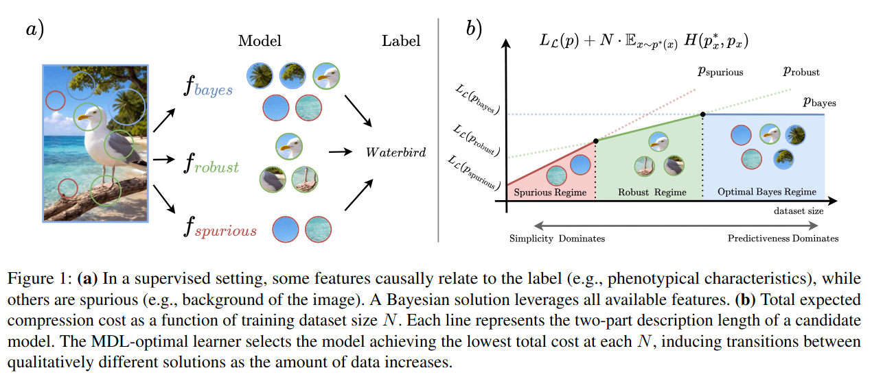
Plots and Observations

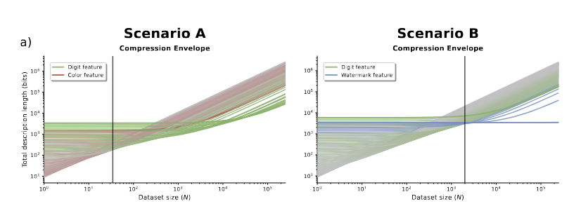Model Complexity/Candidate predictor length vs Dataset size. - As we go to high data regime, the model learns more complex features till it starts overfitting. We observe two regime changes the plots.

• What is the color? - We introduce Digit, Color and Watermark test sets, where the label correlates exclusively with a single feature, measuring the model’s reliance on that specific feature.

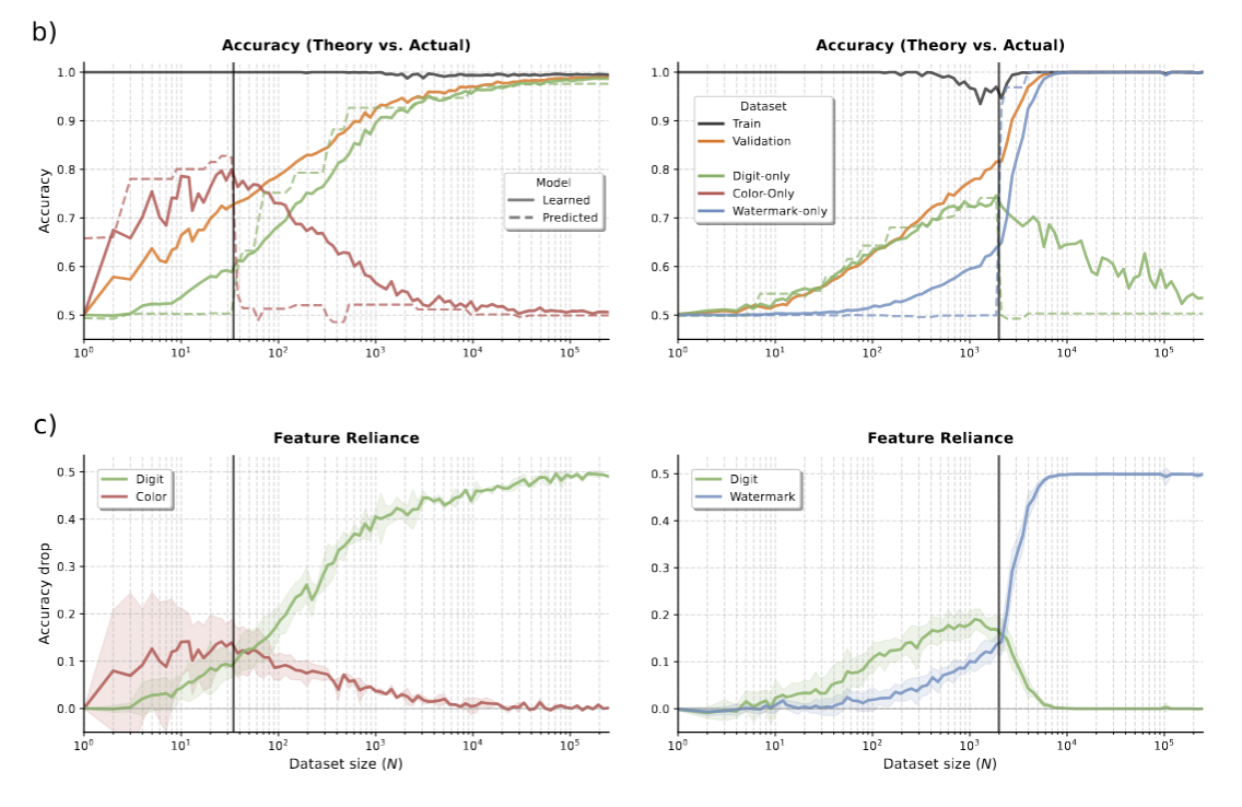
• b) The colored plots for accuracy are just evals on datasets containing one main feature and other featured just being shuffled. e.g color is yellow but digit and watermark are different - there are 1k samples like these.
  • As seen, the core feature(digit is learnt) after an threshold N in the spurious regime test(left) and the watermark is memorised after another threshold in the robust regime(right)
• c) Permutation feature importance: We assess model reliance on each feature by randomly shuffling the values of a single feature of interest (e.g., digit, color, or watermark) across the test set, breaking its correlation with the label while preserving its marginal distribution.
  • HIGHER THE DROP - HIGHER THE IMPORTANCE OF THE FEATURE

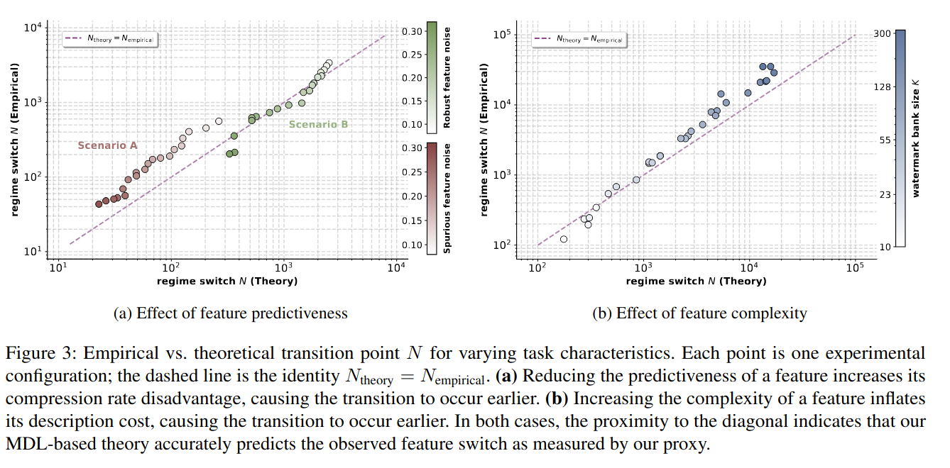
• Feature predictiveness- A measure of the correlation between the feature and the label. The value of the feature essentially. Here,Predictivity is controlled by the noise in data.
• Feature complexity - Complexity refers to how much model capacity and information (in bits) are required to extract, represent, and learn a feature. It is the Price of the Feature. It is controlled by the size of the banks of watermarks corresponding to a label.

Experimental Setup

The experiments use a semi-synthetic visual benchmark derived from Colored MNIST. The core task is a binary classification problem: predicting whether a handwritten digit is smaller than 5 (class $y = 0$) or greater than or equal to 5 (class $y = 1$).

Data Generation Procedure

The dataset is built using the EMNIST digits dataset, which contains 280,000 samples. All images are resized to $32 \times 32$ pixels. Each generated sample simultaneously carries three distinct types of features:

1. Digit Shape (Robust Feature): This is the true causal determinant of the label. The binary label is assigned as $y = \mathbb{I}[d \geq 5] \oplus \text{Bernoulli}(p_{\text{flip}})$, where $p_{\text{flip}}$ represents a label-flipping noise parameter that controls how predictive the digit shape is.
2. Color (Simple Spurious Feature): Digit colors are applied based on the sample’s environment and label. Each sample is randomly assigned to one of two environments $e \sim \text{Bernoulli}(p_e)$, where $p_e$ governs the environment imbalance and controls the predictiveness of the color.
   • In Environment 0: $y = 0$ digits are colored green, and $y = 1$ digits are colored red.
   • In Environment 1: $y = 0$ digits are colored red, and $y = 1$ digits are colored green.
3. Watermark (Complex Environmental Cue): A binary watermark pattern is embedded into the rightmost pixel column of the $32 \times 32$ image. The watermark is drawn uniformly from one of two non-overlapping pre-generated banks of $K$ unique random binary vectors of length $32$ (one bank per environment, $B_0$ and $B_1$). The bank size $K$ controls the complexity of this feature, as the model must memorize all $2K$ patterns to exploit this cue.

Experimental Scenarios

To evaluate how neural networks behave compared to Minimum Description Length (MDL) predictions, two primary configurations of this benchmark are tested:

• Scenario A (Spurious vs. Robust):
  • The watermark is omitted, the robust feature has no noise ($p_{\text{flip}} = 0$), and there is an environment imbalance ($p_e = 0.25$). Here, the color feature is mathematically simpler to learn than the digit feature but is less predictive of the true label.
  • The framework predicts that the network will rely on the simple color feature at low dataset sizes ($N$) before transitioning to the digit feature at higher $N$.
• Scenario B (Robust vs. Bayes-Optimal):
  • The environments are balanced ($p_e = 0.5$), which eliminates any color-label correlation. The robust digit feature is made noisy ($p_{\text{flip}} = 0.15$), setting an accuracy ceiling of 85%. A complex watermark is added with a bank size of $K = 50$.
  • Since the watermark perfectly correlates with the environment, exploiting it allows a “Bayes-optimal” model to achieve higher predictive accuracy, but at the cost of memorizing $100$ distinct random pattern variations (It needs to memorise the entire bank of patterns per environment).
  • The theory predicts the model will prefer the simple digit feature at intermediate $N$ before paying the high complexity cost to transition to the watermark feature at very large $N$.

How the Theoretical Compression Cost is Estimated

To validate the MDL predictions, the authors estimate the two-part description length of different candidate predictors ($p_{\text{spur}}$, $p_{\text{robust}}$, $p_{\text{bayes}}$):

• Fixed Cost (Model Complexity, $L_{\mathcal{L}}(p)$):

  • The authors train a neural network $p_N$ on a custom dataset where all variables except the target feature are randomly shuffled to isolate only that feature.
  • They tightly estimate $L_{\mathcal{L}}(p)$ using prequential coding and apply a blockwise approximation.
    • They have blocks with data boundaries at sizes 1,2,4,8,16,etc.
    • They train on block 0-t1 and then use it to predict samples from t1- t2.
    • Reinit the network and train on 0-t2 and check the error on images in t2.
    • repeated this process block by block till the end.
  • For every single image in your dataset, look up two values:
    • Error A: The error the network made on this image when it was still in training (during the block-by-block step).
    • Error B: The error the final, fully-converged master model makes on this exact same image.
    • Subtract Error B from Error A for every image.
      • Sum up all these differences. This final number is your Model Cost (fixed cost)

• Variable Cost (Data Encoding, $N \cdot \mathbb{E}[-\log p(y|x)]$ ):

  • This measures the remaining randomness not captured by the model and is estimated as the empirical cross-entropy loss evaluated on a held-out test dataset.
    • Evaluate on Test Data: Take your fully-trained “master” model.
    • Run Predictions: Feed a completely separate, clean test set into this model.
    • Get the Average Error: Calculate the average cross-entropy loss across all of these test images.
    • Scale by Dataset Size: Multiply this average test error by your current dataset size N. This is your Data Cost (variable cost).

Neural Network Training Setup

The neural networks representing the empirical learning view are trained using standard Empirical Risk Minimization (ERM):

• Architecture: A Multi-Layer Perceptron (MLP) with two hidden layers of dimension $256$, utilizing ReLU activations and Xavier (Glorot) uniform initialization. The input is a flattened 32x32 RGB image (3072 dimensions).
• Optimization: Standard ERM using the AdamW optimizer with a learning rate of $\eta = 10^{-3}$ and $L_2$ weight decay (regularization) of $\lambda = 10^{-4}$. Batch size is set to $64$.
• Convergence: Models are trained until convergence using early stopping with a patience of 3 epochs and a minimum improvement threshold of $5 \times 10^{-4}$.
• Runs: To minimize variance in small datasets, the authors average results over 10 independent runs for $N \leq 500$ and 3 independent runs for $N > 500$.