#data-efficient-ml paper: openaccess.thecvf.com/content/CVPR2024W/DDCV/papers/He_Large-scale_Dataset_Pruning_with_Dynamic_Uncertainty_CVPRW_2024_paper.pdf

Proposed Ideas

• Generality Easy to learn samples are pruned out and focus is shifted to the hard(high train loss) samples.
• They argue that focus be shifted to uncertain samples rather than hard ones. Because hard ones are often mis-labled or noise data. Most of the information regarding the decision boundary is learned from the uncertain samples.
• They want to prune out a coreset which is subset of the dataset. Models trained on this coreset should be able to achieve comparable generalisation to those trained on the entire data.

Mathematical Notations

The following notations are used to define the dataset and the pruning process:

• $T$: The original large-scale labeled training dataset containing $n$ samples, $\{(x_1, y_1), ..., (x_n, y_n)\}$.
• $S$: The pruned subset (coreset), where $S \subset T$ and $|S| < |T|$.
• $x$: A data point (image) in the $d$-dimensional space $\mathbb{R}^d$.
• $y$: The ground-truth label belonging to one of $C$ classes.
• $k$: The current training epoch ($k \in \{0, ..., K-1\}$).
• $K$: Total number of training epochs.
• $J$: The length of the sliding window used to calculate prediction uncertainty.
• $r$: The pruning ratio, calculated as $1 - \frac{|S|}{|T|}$.
• $\mathbb{P}(y|x, \theta^k)$: The model’s predicted probability for the true label $y$ given input $x$ at epoch $k$.

---

Core Methodology

The algorithm operates in two main phases: calculating uncertainty within a sliding window and then averaging these values to capture training dynamics.

Phase A: Calculating Prediction Uncertainty ($U_k$)

The uncertainty for a sample at a specific epoch $k$ is defined as the standard deviation of its predicted probabilities for the correct label over $J$ successive training epochs:

$$U_{k}(x)=\sqrt{\frac{\Sigma_{j=0}^{J-1}[\mathbb{P}(y|x, \theta^{k+j})-\overline{\mathbb{P}}]^{2}}{J-1}}$$

Where $\overline{\mathbb{P}}$ is the mean prediction probability over those $J$ epochs:

$$\overline{\mathbb{P}}=\frac{\Sigma_{j=0}^{J-1}\mathbb{P}(y|x, \theta^{k+j})}{J}$$

Phase B: Capturing Training Dynamics ($U(x)$)

Rather than relying on a single snapshot, the final Dynamic Uncertainty score $U(x)$ is the average of these sliding-window uncertainties throughout the entire training process: $$U(x)=\frac{\Sigma_{k=0}^{K-J-1}U_{k}(x)}{K-J}$$

Pruning Algorithm (Algorithm 1)

The overall procedure for dataset pruning is as follows:

1. Initial Model Training: Train a deep model $\phi_\theta$ on the full dataset $T$ for $K$ epochs.
2. Collect Predictions: In each iteration, compute and store the prediction $\mathbb{P}(y_i|x_i, \theta)$ for every sample.
3. Compute Scores: Use the stored predictions to calculate the $U_k$ for each sample (starting after epoch $J$) and finally the total dynamic uncertainty $U(x)$.
4. Rank and Select:
   • Sort all training samples in descending order based on their $U(x)$ scores.
   • Select the top $(1-r) \times |T|$ samples to form the pruned dataset $S$.
   • Output the pruned dataset $S$ for future model training.

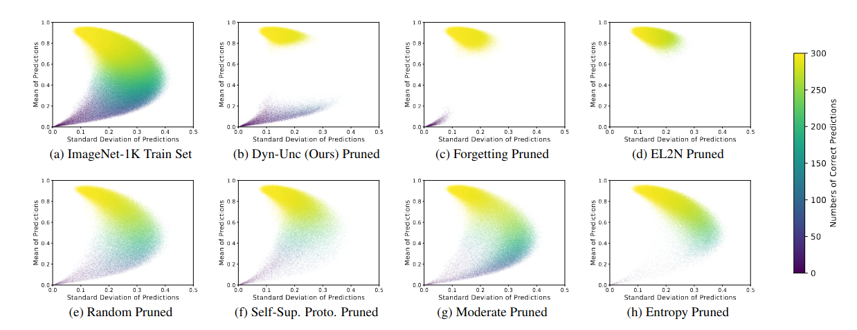The above figure shows the parts of the dataset that are Pruned out. Here Mean prediction refers to the predicted probability of the true label for a data point averaged over the entire training run.

• High mean implies that its easy to learn

• low mean implies its hard

• The X-axis is the std deviation of prediction for a particular data point.

• Notice how only the no variance samples were pruned out from the dataset?

• el2n just focused on pruning out the high mean samples leaving the rest behind.

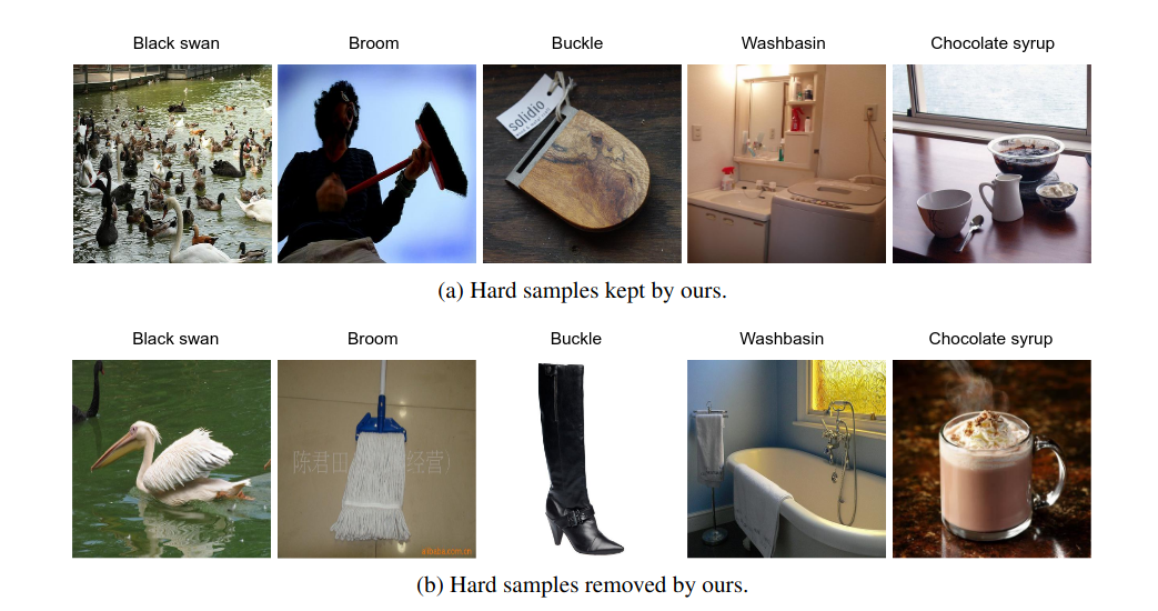
• Interestingly, our dataset pruning method can improve the OOD detection performance slightly, from 21.98% (no pruning) to 22.61% (pruning 30% samples). The possible reason is that dataset pruning prevents models from over-fitting many easy and noisy samples, and thus improves model’s generalisation ability.

Related Work

Deep Learning on a Data Diet