Understanding Visual Feature Reliance through the Lens of Complexity
#compvis #interpretebility #compvis paper: \[2407.06076\] Understanding Visual Feature Reliance through the Lens of Complexity
Key Takeaways
- a new metric for quantifying feature complexity, based on V-information and capturing whether a feature requires complex computational transformations to be extracted.
- They create a dictionary of 10k features based on the penultimate layer representations such that each representation is a linear combination of dictionary vectors
- Define complexity of feature based on the V information
- Define importance of a feature
- Analyse when features are learned during training and where within the network complex features flow.
- simler features tend to bypass the visual heirarchy via residual connections
- Complex features tend to be less important
- Important features become accessible at earlier layers during training
Experiments
- They trained on the repr layer of resnet50 on imagnet.
Generating the Feature Dictionary
Defining Complexity
V- Information
- Define the complexity of a feature and inputs
- Why think about computational effort?
- By explicitly including computational constraints, V-information allows researchers to measure the computational effort required to decode the information, successfully highlighting the massive difference between a feature just existing theoretically in the math and being practically accessible to a neural network.
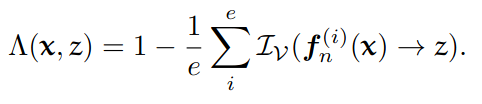
To calculate the final complexity score of a feature ($K(z, x)$), the researchers rely on calculating the V-information at every layer of the neural network: $K(z, x) = 1 - \frac{1}{n} \sum_{\ell} I_{\mathcal{V}}(f_\ell(x) \to z)$.
The elegance of their approach lies in how the V-information equation—which normally measures how hard it is to decode a feature—collapses into a very simple, closed-form solution when the decoder is mathematically restricted. 1. Define the Predictive Family (The “Decoder”) The predictive family, $\mathcal{V}$, represents the computational tool trying to extract the feature $z$. The researchers define this family as a set of linear classifiers that output predictions as Gaussian distributions:
- Without seeing the input data ($\emptyset \to z$): The best it can do is guess a Gaussian distribution centered around a constant mean $\mu$. This is written as $\mathcal{N}(\mu, \sigma^2)$.
- When seeing the input data ($x \to z$): The decoder uses a simple linear transformation matrix ($M$) applied to the input $x$ to predict the mean. This is written as $\mathcal{N}(\psi(x), \sigma^2)$, where $\psi(x) = Mx$.
- To make the math clean, they fix the variance of these Gaussian predictions to $\sigma^2 = \frac{1}{2}$.
2. Set Up the V-Information Equation By definition, V-information is the difference between the uncertainty of the feature alone (V-entropy) and the uncertainty of the feature given the input data (Conditional V-entropy):
$$I_{\mathcal{V}}(x \to z) = H_{\mathcal{V}}(z) - H_{\mathcal{V}}(z \mid x)$$Because the decoder predicts probability distributions, measuring this “uncertainty” means finding the parameters that minimize the negative log-likelihood of the Gaussian distributions.
3. Substitute the Gaussian Math When you plug the standard Gaussian probability density formula ($\frac{1}{\sqrt{2\pi\sigma^2}} e^{-\frac{(z-\mu)^2}{2\sigma^2}}$) into the negative log-likelihood equation, something highly convenient happens: the natural logarithm ($\log$) cancels out the exponential function ($e$).
The equation simplifies to just minimizing the squared error terms:
$$I_{\mathcal{V}}(x \to z) = \inf_{\mu \in \mathbb{R}} \mathbb{E}_{z} \left[ \frac{(z-\mu)^2}{2\sigma^2} \right] - \inf_{\psi \in \Psi} \mathbb{E}_{x,z} \left[ \frac{(z-\psi(x))^2}{2\sigma^2} \right]$$4. Factor Out Variance and $R^2$ Next, you can factor out the $\frac{1}{2\sigma^2}$ from both terms. Notice that the first term, $\inf_{\mu} \mathbb{E} \left[ (z-\mu)^2 \right]$, is exactly the mathematical definition of the baseline statistical variance of the feature, denoted as $\text{Var}(z)$.
If you factor $\text{Var}(z)$ out of the entire equation, you get:
$$I_{\mathcal{V}}(x \to z) = \frac{\text{Var}(z)}{2\sigma^2} \left( 1 - \frac{\inf_{\psi} \mathbb{E} \left[ (z-\psi(x))^2 \right]}{\text{Var}(z)} \right)$$The massive fractional term on the right side of the parenthesis is exactly the formula for the fraction of unexplained variance. Therefore, $1$ minus that term is exactly the Coefficient of Determination ($R^2$).
5. The Final Collapse Finally, remember that the researchers intentionally fixed the Gaussian variance $\sigma^2$ to $\frac{1}{2}$. Because $\frac{1}{2(1/2)} = 1$, the leading fraction disappears.
The complex information-theoretic equation elegantly collapses into:
$$I_{\mathcal{V}}(x \to z) = \text{Var}(z)R^2$$Coefficient of Determination
- It quantifies the fraction of the total variance of z that is predicted by the classifier. How this finalizes the Complexity Score: Because the data in neural networks is typically centered and scaled, the baseline variance $\text{Var}(z)$ is generally around 1. This means the V-information score at any given layer is essentially just bounded by the linear $R^2$ score.
By averaging this V-information across all layers and subtracting it from 1, the final complexity score ($K(z, x)$) lands cleanly in the range of . A score near $0$ indicates a simple feature that the linear Gaussian probe could easily decode across the whole network, while a score near $1$ indicates a highly complex feature that completely stumped the linear probe.
Time to decode
- So V-info here tells us the mutual information between the penultimate layer representation and the ultimate feature values.
- So if a representation can be decoded into a particular feature z earlier on in the training, then the V-info would be closer to 1 since the starting epochs. Hence the average over epochs would be close to 1. and Hence 1 - the avg would yield a value close to 0 => lower time to decode.
Importance
importance measure Γ(zi) quantifies the average contribution of the i-th feature to the class-specific logit.
Findings
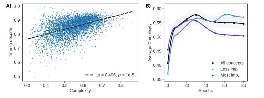
- Strong Correlation betweeen complexity and required temporal span for its decoding
- Complexity of important features decreases with epochs.