This blog is a detailed overview of one of my favourite projects of creating a superhuman player for the game of Black Hole. This was a passion-project of mine which I had been planning for some time and finally got around to implementing a few months ago. AlphaZero was a pioneering work in the field of Reinforcement Learning and hence my motivation to implement it for a game. I learnt a lot over the course of doing this and this is my small attempt to explain the theory behind the work and what I tried to do.
Introduction to RL
Reinforcement learning is a subfield of deep learning which focuses on teaching models(termed as agents) by making them interact with some environment. The main idea is very heuristic, the model gets conditioned to perform only those actions which are beneficial to it.
How is this “benefit” actually defined? This is done with the help of reward functions - a function $R(s, a, s^\prime)$ that takes the current state $s$, the action $a$ taken by the agent, and the next state $s^\prime$ , and returns the reward for that action.
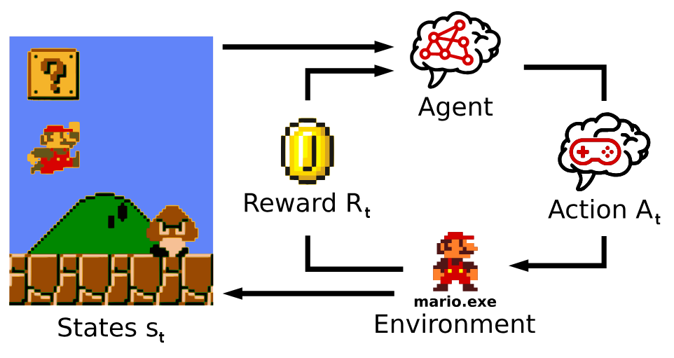
The reinforcement learning cycle.
As shown above, the agent interacts with the environment, gets some rewards, trains itself based on rewards and repeat. Now while idea is simple in theory, designing reward functions and RL traininig frameworks which cater to our needs is a challenging task.
Rules of Black Hole
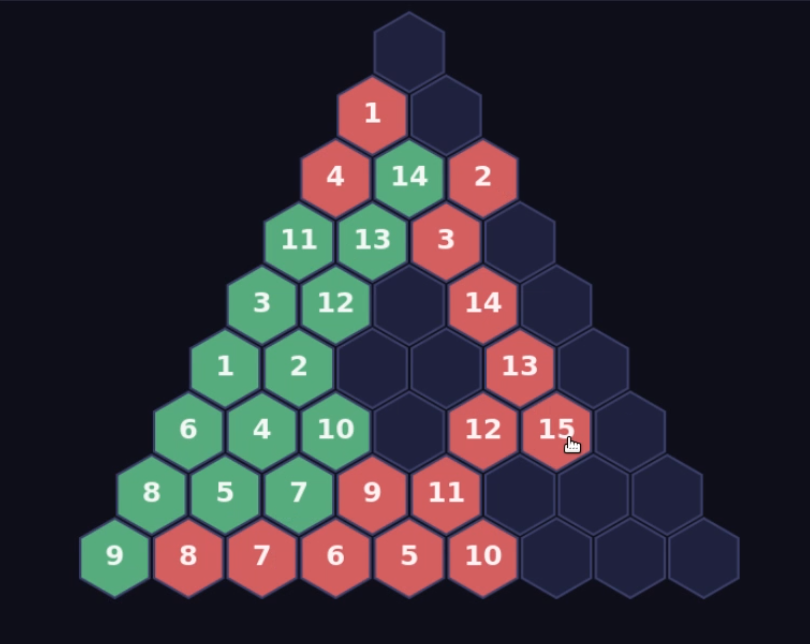
Black Hole is a strategic tile-placement game played on a triangular grid. It was designed by the members of the DTU chapter of the Indian Game Theory Society(IGTS). I came across this because of my involvement with my university’s chapter of IGTS - the KGPian Game Theory Society. Traditionally it has 6 rows, but I had to expand it to 9 rows for more stable training. It has 45 empty spaces in total.
The game of Black Hole
How to Play
The Setup: Two players each receive 22 tiles numbered 1 to 22. The board starts empty.
The Turn: Players take turns placing one tile onto any empty spot. You must play your tiles in ascending numerical order (1, then 2, then 3, up to 22).
The Black Hole: Because 44 tiles are placed onto a 45-space board, exactly one space is left empty at the end. This becomes The Black Hole.
Scoring
The Black Hole “sucks in” neighboring tiles. Scoring is calculated in concentric rings radiating outward from the hole (Ring 1 is immediate neighbors, Ring 2 is the next layer out, etc.).
Your goal is to get sucked in as little as possible. The player whose tiles in Ring 1 have the lowest sum wins instantly. Ties are broken by evaluating Ring 2, and so on.
Google Deepmind’s AlphaGo and AlphaZero
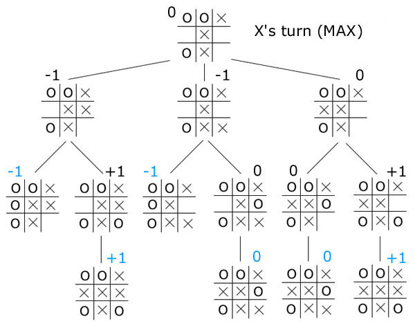
For most of computing history, game-playing AI was built on a deceptively simple idea: search. The logic goes like this: any game has a defined set of states and transition rules. Given enough time and processing power, you could enumerate all possible futures, assign a value to the terminal state (win/loss/draw), and trace backward to assign a value to every preceding state. The optimal strategy is simply to choose the move that leads to the highest-valued state. This is called minimax algorithm.
The game of Tic-Tac-Toe represented as a game tree. (source: https://www.yosenspace.com/posts/computer-science-game-trees.html)
Chess engines like Stockfish perfected this approach, checking millions of positions per second, guided by handcrafted evaluation functions tuned by human grandmasters. It worked extraordinarily well, but it required too much human intervention.
But this approach was grossly insufficient for games like Go which had a massive action space for each state, hence a branching factor much larger(~7-8x) than that of chess. And give that the search space grows by the order of branching factor raised to the power of no. Of moves in the game ($b^d$), it’s computationally infeasible to find the optimal move for games like Go.
AlphaGo was the pioneering work which tried to solve this problem. It had a two-part insight. First, a policy network learned to predict which moves strong players would make, dramatically pruning the search tree. Second, a value network learned to estimate the probability of winning from any given board state, replacing handcrafted evaluation. Both networks were trained initially on a dataset of human expert games, and then refined through self-play using reinforcement learning.
In October 2015, AlphaGo played its first game against the reigning three-time European Champion, Fan Hui. AlphaGo won the first ever match between an AI system and Go professional, scoring 5-0.
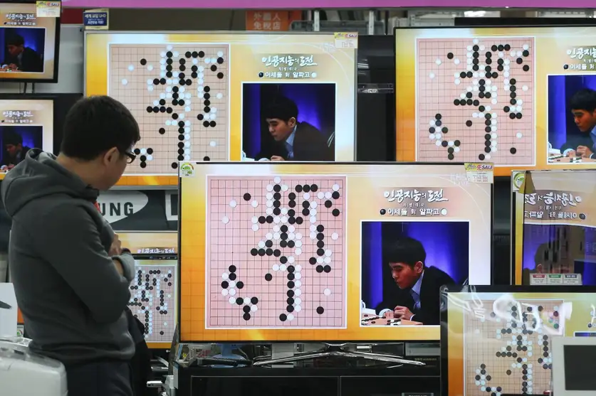
Lee Sedol vs AlphaGo. (source: https://www.newscientist.com/article/2518450-the-moment-that-kicked-off-the-ai-revolution/)
AlphaGo then competed against legendary Go player Lee Sedol — winner of 18 world titles, and widely considered the greatest player of that decade. AlphaGo’s 4-1 victory in Seoul, South Korea, in March 2016, sent shockwaves across the globe. It demonstrated that deep learning could internalize strategic intuition that no one had successfully written down.
AlphaZero, published in 2017, took this further by stripping out the human data entirely. There were no expert games and no domain-specific heuristics - just the rules of the game and time to play itself. It achieved this with the help of a modified Monte Carlo Tree Search Algorithm paired with its Policy and Value Networks which essentially guided the exploration and search process.
Within hours of training, AlphaZero surpassed AlphaGo; within days, it exceeded the best classical engines in Go, Chess, and Shogi simultaneously — using the same algorithm for all three!
Classical Self-Play
How does your AI agent learn to play a game without having any prior experience or expert data as reference? The answer is that if creates its own data through self-play and trains on it – gradually improving its strategy in the process.
The most basic form of self-play is to make your trainable model play out a large number of games against a frozen version of itself. You store these games into a memory buffer and then use these as data to train your model to understand which strategy is better. You also keep updating your frozen opponent model with newer versions of your main agent as it keeps learning.
Alpha Go also used a similar strategy but instead of starting from scratch (random policy), it was first trained on a ton of expert human games of Go. After that it was trained to further improve its strategic thinking via self-play.
Monte Carlo Tree Search
The Monte Carlo Tree Search(MCTS) is a heauristic search algorithm which helps us find near optimal moves by partially observing the future from a particular game state. It is method that helps us effectively navigate through the decision trees of problems with very large decision spaces like Go(which has $10^{170}$ possible game states).
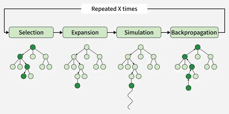
The four steps of the MCTS algorithm. (source: https://www.geeksforgeeks.org/machine-learning/monte-carlo-tree-search-mcts-in-machine-learning/)
MCTS works by randomly sampling the search space through playouts. It does many playouts where it randomly simulates(random decisions) the entire game to the end and keeps expanding a temporary game tree from it’s root current game state. The final result of each playout is then used to update the statistics of the nodes visited during that playout and helps us get an estimate of which nodes lead to better outcomes. Now, the way decisions are made before the random sampling is determined by the the objection function called Upper Confidence Bound (UCB).
where $W$ is the number of wins for a node, $N$ is the number of simulations for a node, and $c$ is the exploration parameter.
Each MCTS Sampling Iteration involves the following steps:
Selection - Starting at the root(current game state) node, we compute the UCB score for all its children in the current game tree(using the current win-visit stats) and navigate down the current game tree by greedily selecting the node with the highest UCB score.
Expansion - Once we reach a node(during the above traversal) that has not been fully expanded(has legal moves which have not been visited), we expand it by adding one of its unvisited child nodes to the tree(because UCB for the unvisited node is $\infty$).
Simulation - From the expanded node, we simulate the game to the end by randomly selecting moves.
Backpropagation - Once we reach a terminal state, we backpropagate the result to the root node by updating the statistics of all the nodes visited during the selection and simulation steps.
///
Note:
MCTS iterations involve exploring both the current player’s as well the opponents decisions. Alternate layers of the game tree will be formed by the opponent’s decisions. Hence, during backpropagation we have to ensure that the win score reflects this difference. For example, if the terminal state results in the current player winning, the player nodes get +1 win score and opponent nodes get -1 win score and vice versa.
After some N iterations, the current player makes the move which corresponds to the most visited child node of the root state. The game then moves on to the opponent’s turn and the same process is repeated from their perpective with the new game state as the start of a new MCTS tree.
The following visualization shows the MCTS process on a simple game. Players take turn placing their coins in any of the four available slots. The goal of the game is to not have your coins in adjacent slots. Whoever does that loses the game.
step 1 / 8
selection
How AlphaZero Actually Learns
By this point we’ve covered MCTS and how it builds a search tree to make decisions. Now the question is: how does AlphaZero get good at this? The answer is a tight feedback loop between a neural network and a modified MCTS — each one making the other better.
The Neural Network
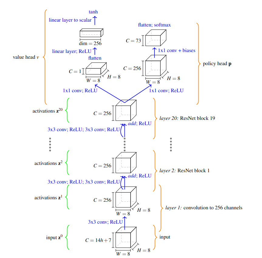
AlphaZero uses a single deep residual network (ResNet, 20 blocks) that takes a board state as input and outputs two things simultaneously:
p — a probability distribution over all legal moves (the policy head)
v — a scalar in [-1, 1] estimating the expected outcome from this position (the value head)
The input is an tensor encoding the current board plus states from the last few moves (say 4), always oriented from the perspective of the side to move. Having the history helps the network to detect patterns like threefold repetition or gradual piece development although for my implementation I only used the current board state. Having a history seems to be more important for games like chess, however that ablation still needs to be done for the game of Black-Hole.
///
Network Architecture
The neural network architecture of AlphaZero (source: https://arxiv.org/pdf/2111.09259)The value and policy outputs are generated by two separate heads. However these heads aren't independent, they share a representation generated by the preceeding residual layers, which means learning to evaluate positions also improves move selection and vice versa. I believe this coupled nature of the heads is one of the key aspects of AlphaZero's success.
The Training Loop
Training is a continuous cycle of three things happening in parallel:
1. Self-play data generation
The network plays games against itself. At every position $s_t$ in every game, it runs N (100 for Black-Hole) MCTS simulations to produce an improved move distribution $\pi_t$. It then samples a move from $\pi_t$ and plays it. This continues until the game ends with outcome $z \in \{+1, 0, -1\}$.
Every position from the game gets stored in a replay buffer as the tuple $(s_t, \pi_t, z)$ — board state, the MCTS-improved policy, and the final game result. The buffer holds the last 4K positions. Now to speed up the data collection, we run multiple self-play games in parallel every iteration and then store the data from all of these in the buffer.
2. Gradient Updates
Mini-batches of size 512 are sampled from the replay buffer and used to minimize the loss function:
$$l = (z - v)^2 - \pi^T \log p + c||\theta||^2$$
Three terms:
$(z - v)^2$ : Mean Squared Error between the network’s value prediction $v$ and the actual game outcome $z$. This trains the value head to be an accurate position evaluator.
$-\pi^T \log p$ : Cross-entropy between the raw network policy $p$ and the MCTS-improved policy $\pi$. This guides the policy head to output better action probabilities, ones that are closer to what MCTS determined to be good. Equivalent to minimizing the KL-divergence between $p$ and $\pi$.
$c||\theta||^2$ : L2 regularization to prevent the weights from blowing up.
SGD with momentum 0.9, initial learning rate 0.2, decayed by 10× at 100k, 300k, 500k, and 700k steps, for a total of 1 million gradient steps.
3. Dynamically Improving Matchups
Every 10 iterations, we do a few evaluation run between the current model and the previous best model. If the avg win-rate of the current model is greater than 60%(55% in the original paper), we update the previous best model to be the current model.
Due to noisy training dynamics, I also added an extra criteria of having to win for atleast 5 consecutive evaluations for the opponent to get replaced.
From Raw Policy to Improved Policy: Guided MCTS
The raw policy from the Policy Network is used as a crude guide for the MCTS. We run around 40 simulations for at each move of the game to get the improved Policy. The process is as follows:
Step 1 — Initialize
The network evaluates the root position, giving prior probabilities $p$ over all legal moves. Before search begins, Dirichlet noise is injected into these root priors:
where $\varepsilon = 0.25$. This forces the search to occasionally explore moves the network thinks are weak — without it, the self-play games would be too repetitive and the network would never discover surprising lines. This noise is only applied at the root, not deeper in the tree.
Step 2 — MCTS Simulations
Each simulation traverses the tree from root to a leaf, governed by the PUCT algorithm. To understand exactly how the search tree is dynamically built, let’s trace the first three simulations:
Simulation 1 (Root Evaluation): We start at the root node. Because it hasn’t been expanded, selection stops immediately. The board state is passed to the neural network, which outputs the naive policy probabilities $P(s,a)$ and a value estimate $v \in [-1, 1]$. We create child nodes for all valid moves, initialize their priors using the network policy, and backpropagate $v$ to the root, increasing its visit count $N(s)$ to 1. (Note: To ensure exploration, the Dirichlet noise is injected into these root priors right after this initial evaluation).
Simulation 2 (Prior-Driven Selection): Starting at the root again, we must pick a child using the PUCT score:
$$\text{Score}(s, a) = Q(s, a) + C_{\text{puct}} \cdot P(s, a) \cdot \frac{\sqrt{N(s)}}{1 + N(s, a)}$$
Since all children currently have 0 visits, $Q(s, a) = 0$. The score is entirely dominated by the network’s prior $P(s, a)$. The search blindly trusts the network and selects the move with the highest naive probability. We traverse to this new leaf, evaluate it with the neural network, expand its children, and backpropagate its value $v_{leaf}$ up the tree (flipping the sign at each level since turns alternate).
Simulation 3 (Exploration vs. Exploitation): Back at the root, the previously selected child now has 1 visit and a non-zero $Q$-value. Its exploration term decreases. We now face a choice:
Exploit: If the previous leaf resulted in a highly favorable $Q$-value, its total score might still beat the unvisited siblings. We select it again and dive deeper into that branch.
Explore: If the evaluation was poor (negative $Q$), or an unvisited sibling has a highly competitive prior $P(s, a)$, the search pivots and explores a new action.
This process repeats for N simulations. Early on, the exploration bonus ($U$) dominates and the search follows the network’s intuition. Over time, as visits accumulate, the actual simulation results ($Q$) take over. Crucially, no random rollouts are used—the neural network’s value head replaces them entirely at the leaf nodes.
Step 3 — Extract the improved policy
After N simulations, the improved policy $\pi$ is computed from visit counts:
Temperature $\tau = 1$ during training (preserving the full distribution), and $\tau \to 0$ during evaluation (collapsing to the most visited move deterministically).
///
Why is $\pi$ better than $p$?
The raw policy $p$ is the network’s immediate intuition about the position — it hasn’t looked ahead at all. MCTS acts as a policy improvement operator by exploring hundreds of continuations, catching tactical traps several moves deep, and adjusting visit counts accordingly. A move that looks fine to the network but leads to a lost position 6 moves later will have low $Q$, get visited less, and end up with low $\pi$. The visit count distribution encodes the network’s intuition corrected by lookahead.
Testing the Model
Now that the model has been trained, we can now test it out against other players. But how to do does the model take decisions? We now have two options, we can use either just the trained policy head to make the decisions given a state $s$, or we can use the MCTS algorithm to derive the improved policy $\pi$ using the trained policy head and value head to make the decisions given a state $s$.
In the following clip, I am playing against one of the my trained models which is using just the training policy network to make decisions (argmax of the output logits).
As you can see even this simple implementation is quite strong. It can play on par with intermediate level players. One thing to be noted thought is that the model’s strategy is entirely deterministic. I had tried a more stochastic inference with top-p sampling but it did not perform that well. I also did not put that many training hours into this which might be the reason it doesn’t perform as well as it could have.
Future Work
My implementation was a pretty naive one and there are quite a few things I would like to explore with this project (whenever I find time to that is):
Retrain for more hours for better robustness across stochastic policies.
Modifying the inference pipeline for improved sampling of actions.
Prepare a elo based ranking setup for comparing different models with different configurations e.g mcts vs no-mcts vs random vs human policy.
Try having a history of states as input instead of a single state and observe if that leads to any improvements.
Thank you for reading. Please let me know if you have any suggestions or questions!