Diffusion Models for Dummies: Getting Started
Table of Contents
Generative AI has been the buzz and face of AI industry for the last few years. Particularly image and video generative models. How do they models generative an image when given a prompt? But how exactly does a model take in text prompt and transform it into a visual output catering to the context of that prompt?
This is where diffusion comes in ! One of the most amazing model architectures and training methodologies in modern AI.
My intention with this blog will be to give you a intuitive overview of some of the math and the training workflow of diffusion along with a hands-on implementation at the end. While I will go over the necessary math involved, it does not even start to cover the entirety of this beautiful topic. However, it should be good enough to get a rough idea of the underlying principles and should(hopefully) motivate you to dive deeper.
Here are the topics that we will follow:
- Images as Samples of a distribution
- A Model as an Approximation for a Distribution
- Diffusion - Forward Process - Generating Training Data
- Diffusion - Reverse Process - Generating Image from Noise
- Implementation
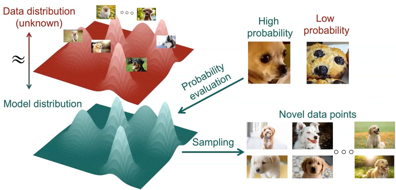
Images belong to a Distribution
Since diffusion based models rely on the idea of transforming a probability distributions and then sampling from them, it is judicious to first understand how images can be seen as samples from some probability distribution.
Any image is just a grid of pixels and each pixel is just a tuple of RGB values. If you consider an image to be a set of variables then you can create any image of resolution HxW with 3xHxW independent continuous variables ranged between 0-255(or some other common scale). For a typical image generator, generating the image is like sampling from a joint probability distribution of all these variables.
Ofcourse, if the distribution is just some standard distribution like the Gaussian then you will just get a noisy incoherent image. But given that the distribution is a relevant and useful one , the kind of images you want will have high probability densities and the useless irrelevant ones will have lower.
During training also we like to assume that all the images of our image dataset belong to some joint probability distribution over the variables and we train our model to learn this ideal distribution from the training data points.
Neural Networks as an Approximation
It is very difficult to arrive at a closed form solution for getting this probability distribution given the very high dimensionality of the sample space. Hence we use neural networks to approximate this distribution function.
For a discrete sample space, for example in the case of classification problems, we have fixed set of classes into which we need to segregate an image. So typically what we do is we train the model to take in an input and give a probability mass function over the different classes. Then we choose the class with the highest probability as the identified class of the input.
However in the case of image generation we are dealing with a continuous space and so the approximated function has to be a probability density function over this sample space. How can this be done?
One naive approach would be to try training a model to give a real value for each possible image pixel combination which sums to 1 over the entire space. But there is no way to ensure the summation property other than to divide the ouput by the sum/integral Z over the sample space; which is computationally infeasible for even moderately sized sample spaces.
$$ Z = \int_{x} f(x) dx \quad\quad p(x)=\frac{1}{Z} f(x) $$The general practice that is followed and works out well is to use NNs to approximate the target distributions using already known probability distributions and using the NN to approximate their defining parameters(mean and variance). For instance, the most standard practice is to use the Gaussian Distribution due to a lot of good properties, which I won’t discuss here.
Therefore, we define the network as
A neural network model with parameters $\theta$ that approximates the $\mu$ and $\Sigma$ of the required multivariate normal distribution.
Diffusion for Image Generation
Denoising Reverse Process
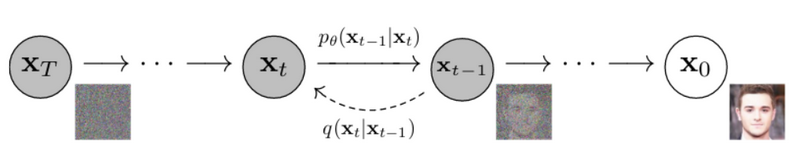
Now in diffusion we don’t exactly find the required probability distribution directly. Instead we follow an iterative process of slowly transforming a starting noisy distribution into the required final distribution. Why is this done? A simple explanation would be, it just works better for the practical scenarios of approximating non-linear functions in high dimensions.
The theoretical diffusion sampling process (the generative Markov chain) is defined by Gaussian transitions
$$ p_\theta(x_{t-1} | x_t) = \mathcal{N}(x_{t-1}; \mu_\theta(x_t, t), \Sigma_\theta(x_t, t)) $$but in practice we consider a only time-dependent variance $\Sigma_\theta(x_t, t) = \Sigma_t$. Learning the variance is mathematically “heavy” and can make training unstable. Early research found that simply following the same “amount” of noise used in the forward process works remarkably well.
$$ p_\theta(x_{t-1} | x_t) = \mathcal{N}(x_{t-1}; \mu_\theta(x_t, t), \Sigma_t) $$At each step the model takes the previous noisy image $x_t$ and calculates the mean for the previous image $x_{t-1}$ and then samples $x_{t-1}$ from the distribution $\mathcal{N}(\mu_\theta(x_t, t), \Sigma_t)$.
Now, we don’t ask the neural network to spit out $\mu$ directly because that’s a difficult learning task.
Instead we use use something called reparameterisation trick to get the values. We use the neural network to predict a noise amount $\epsilon_\theta$ and then use that to approximate the $\mu_{\theta}$ value.
$$\mu_\theta(x_t, t) = \frac{1}{\sqrt{\alpha_t}} \left( x_t - \frac{\beta_t}{\sqrt{1 - \bar{\alpha}_t}} \epsilon_\theta(x_t, t) \right)$$Notice that the model takes in input $x_t$ and t; we will get back to this a bit later. The alpha and beta values are just fixed values depending on the noising schedule that is being followed.
Why do we do this reparameterisation? - Because it makes the training much more stable - similar to how teaching ResNets to predict the change in input is easier for the model than predicting the output estimate. If you are curious why then refer to this paper.
Now given a trained model with parameters $\theta$ , the sampling algorithm for generating an image from the target distribution is as follows:
- Initialize: Start with $x_T \sim \mathcal{N}(0, \mathbf{I})$ (pure white noise).
- Iterate: For $t = T, T-1, \dots, 1$:
- Sample random noise: $z \sim \mathcal{N}(0, \mathbf{I})$ if $t > 1$, else $z = 0$.
- Predict the noise: Pass the current image $x_t$ and the time step $t$ into your model to get $\epsilon_\theta(x_t, t)$.
- Compute the Mean ($\mu_\theta$): This is the “de-noised” version of the current image. $$\mu_\theta(x_t, t) = \frac{1}{\sqrt{\alpha_t}} \left( x_t - \frac{\beta_t}{\sqrt{1 - \bar{\alpha}_t}} \epsilon_\theta(x_t, t) \right)$$
- Update the Image: Calculate the next step $x_{t-1}$ by adding back a tiny bit of controlled variance ($\sigma_t z$) to keep the process stochastic: $$x_{t-1} = \mu_\theta(x_t, t) + \sigma_t z$$
- Result: $x_0$ is your generated image.
This reverse process is summarised in the image below. The sample in red is slowly transformed to a sample from the target distribution over multiple timesteps.
Reverse Diffusion: Skewed Modes
Samples($x_T$) from the initial standard Gaussian distribution(top) get slowly transformed into samples($x_0$) of the target distribution(bottom) over $T$ steps.
(Please reload the page if object not working properly)
This algorithm essentially starts with a single sample from a random distribution and then iteratively transforms the distribution to the target distribution over T steps such that the sample gets transformed to a sample from the target distribution and since in the target distribution only the coherent samples have high probabilities , the final sample should also be coherent and desirable.
The Forward Process and Training
Now that you understand(hopefully) the process of generation of an image via diffusion, we can discuss how these models can be trained.
While there has been a multitude of training methods catering to diffusion and similar architectures, I will be going over the most well-known one which was discussed in the foundational paper of DDPM.
Since we were using the trained model to predict the noise of a given image + timestamp input, we will need to create data to serve this purpose and train it accordingly with some loss function. How do we make the training data for this? We make use of any image dataset and start adding noise at different intensities to the given image!
But we don’t do it in any arbitrary manner, rather we do a time-scheduled addition, hence the “t” in the model input.
In the forward process, we gradually add Gaussian noise to an image step by step. We control how much noise is added at each step using a variance schedule $\beta_t$. If we define $\alpha_t = 1 - \beta_t$, the single-step transition from $x_{t-1}$ to $x_t$ is defined as:
$$x_t = \sqrt{\alpha_t} x_{t-1} + \sqrt{1 - \alpha_t} \epsilon, \quad \epsilon \sim \mathcal{N}(0, \mathbf{I})$$If we had to do this iteratively to generate a noisy image at step $t$, it would be very slow during training. Fortunately, we can recursively expand this formula to sample an image $x_t$ at any arbitrary timestep $t$ directly from the clean image $x_0$, without iterating through all previous steps:
$$x_t = \sqrt{\bar{\alpha}_t} x_0 + \sqrt{1 - \bar{\alpha}_t} \epsilon, \quad \epsilon \sim \mathcal{N}(0, \mathbf{I})$$Where:
- $\bar{\alpha_t} = \prod_{i=1}^t \alpha_i$ (the cumulative product of the noise schedule)
- $\epsilon$ is the “ground truth” noise we injected.
Forward Diffusion Process
Drag the slider to add Forward Gaussian Noise ($q(x_t | x_{t-1})$) to the original image data.
We provide the model (usually a U-Net) with the noisy image $x_t$ and the current timestep $t$. The model’s job is to predict the noise $\epsilon$ that was used to corrupt $x_0$.
What is the most simple loss function you can think of that might be used here? We are predicting a continuous value! This is just regression on the noise values. Therefore, a sane choice would be the Mean Squared Error ($L_2$ norm) between the true noise $\epsilon$ and the predicted noise $\epsilon_\theta$:
$$\mathcal{L}_{simple}(\theta) = \mathbb{E}_{t, x_0, \epsilon} \left[ \| \epsilon - \epsilon_\theta(x_t, t) \|^2 \right]$$///Why $L_2$?
Mathematically, minimizing the $L_2$ error in noise prediction is equivalent to maximizing the Evidence Lower Bound (ELBO) under the assumption that the reverse transitions are Gaussian. Maximizing the ELBO is what ensures that our approximation of the true distribution is as close as possible to the true distribution.
The Training Algorithm:
- Sample a clean image $x_0$ from your dataset.
- Pick a random timestep $t$ between $1$ and $T$ (e.g., $t=450$ out of $1000$).
- Generate random noise $\epsilon$ and mix it with $x_0$ using the formula above to create $x_t$.
- Pass the noisy image $x_t$ and the timestep $t$ to the model and get the predicted noise $\epsilon_\theta(x_t, t)$.
- Compare the predicted noise with the actual noise $\epsilon$ using Mean Squared Error ($L_2$ norm) and calculate the loss.
- Optimise: Take a gradient descent step to minimize the loss.
- Repeat for a number of epochs.
Implementation
First define the hyper-parameters and device. I will be using Pytorch for this implementation. I would suggest using a GPU since training on a CPU would take a lot of time. You may use Google Colab or Kaggle notebooks for this.
import torch
import torch.nn as nn
import torch.nn.functional as F
from torch.utils.data import DataLoader, ConcatDataset
from torchvision import datasets, transforms

T = 500  # Total number of diffusion steps
BETA_START = 0.0001
BETA_END = 0.02

# Flowers102 are RGB natural images; use a slightly larger size than MNIST
IMAGE_SIZE = 64
CHANNELS = 3  # 3 for RGB (Flowers102)
BATCH_SIZE = 32
LEARNING_RATE = 1e-3
EPOCHS = 100
TIME_DIM = 64

device = "cuda" if torch.cuda.is_available() else "cpu"
print(f"Using device: {device}")def get_dataloader():
transform = transforms.Compose([
transforms.Resize((IMAGE_SIZE, IMAGE_SIZE), antialias=True),
transforms.ToTensor(),
transforms.Normalize((0.5, 0.5, 0.5), (0.5, 0.5, 0.5)),
])
root = "./data"
train_ds = datasets.Flowers102(root, split="train", download=True, transform=transform)
val_ds = datasets.Flowers102(root, split="val", download=True, transform=transform)
dataset = ConcatDataset([train_ds, val_ds])
dataloader = DataLoader(
dataset,
batch_size=BATCH_SIZE,
shuffle=True,
num_workers=2,
pin_memory=(device == "cuda"),
)
return dataloader
betas = torch.linspace(BETA_START, BETA_END, T).to(device)
alphas = 1.0 - betas
alpha_bars = torch.cumprod(alphas, dim=0)
if device == "cuda":
torch.cuda.manual_seed_all(42)
betas = betas.to(device)
alphas = alphas.to(device)
alpha_bars = alpha_bars.to(device)
sqrt_alpha_bars = torch.sqrt(alpha_bars)
sqrt_one_minus_alpha_bars = torch.sqrt(1.0 - alpha_bars)
dataloader = get_dataloader()Before we can train, we need to pre-calculate our “noise schedule.” These $\alpha$ and $\beta$ values are the knobs that control how much noise is added at each step. By calculating the cumulative products ($\bar{\alpha}$) upfront, we can jump from a clean image ($x_0$) to a noisy version at any timestep $t$ in a single step, rather than looping $t$ times.
To keep things simple, I’m using the Flowers102 dataset. It’s small enough to train relatively quickly but diverse enough to show that the model is actually learning something interesting. We resize everything to 64x64 and normalize the pixels to the range [-1, 1]. This is important because our model will be predicting noise that also lives around that range(due to sampling from the standard Gaussian distribution).
def forward_diffusion_sample(x0, t, device=None):
    if device is None:
        device = x0.device
    t = t.to(device)

    s_alpha_bar = sqrt_alpha_bars.to(device)[t].unsqueeze(-1).unsqueeze(-1).unsqueeze(-1)
    s_one_minus_alpha_bar = sqrt_one_minus_alpha_bars.to(device)[t].unsqueeze(-1).unsqueeze(-1).unsqueeze(-1)
    noise = torch.randn_like(x0, device=device)
    xt = s_alpha_bar * x0 + s_one_minus_alpha_bar * noise

    return xt, noise
This function is our Forward Process. It takes a clean image and a timestep value $t$, then “corrupts” the image by mixing it with random noise at that corresponding timestep $t$ based on the noise schedule $\beta_t$.
def get_time_embedding(t, dim):
    """Sinusoidal Positional Encoding for time."""
    inv_freq = 1.0 / (10000 ** (torch.arange(0, dim, 2).float() / dim))
    sin_emb = torch.sin(t.unsqueeze(-1) * inv_freq.to(t.device))
    cos_emb = torch.cos(t.unsqueeze(-1) * inv_freq.to(t.device))
    emb = torch.cat([sin_emb, cos_emb], dim=-1)
    return emb
As mentioned before the model predicts the noise at a given timestep $t$ from the input noised image. Denoising at step $t=999$ (almost pure noise) is very different from denoising at $t=5$ (almost clean). However we don’t just pass the timestep $t$ directly as an integer input to the model.
Instead a good practice is to encode the timestep $t$ into a vector embedding representation. Here we use Sinusoidal Positional Encodings—the same stuff used in Transformers—to turn a single integer $t$ into a rich vector that the neural network can understand.
def _pick_gn_groups(channels: int) -> int:
    for g in (32, 16, 8, 4, 2, 1):
        if channels % g == 0:
            return g
    return 1


class ResBlock(nn.Module):
    def __init__(self, channels: int):
        super().__init__()
        g = _pick_gn_groups(channels)
        self.norm1 = nn.GroupNorm(g, channels)
        self.conv1 = nn.Conv2d(channels, channels, 3, padding=1)
        self.norm2 = nn.GroupNorm(g, channels)
        self.conv2 = nn.Conv2d(channels, channels, 3, padding=1)

    def forward(self, x):
        h = self.conv1(F.gelu(self.norm1(x)))
        h = self.conv2(F.gelu(self.norm2(h)))
        return x + h
For the “brain” of our model, we use Residual Blocks. If you’ve seen ResNets, this looks familiar. The idea is to let the gradient flow easily through the network by adding the input back to the output of the convolutional layers. We also use Group Normalization instead of Batch Norm, as it tends to be more stable when working with smaller batch sizes and generative tasks.
class UNet(nn.Module):
    def __init__(self, in_channels, out_channels, time_dim=TIME_DIM,  base_channels: int = 32):
        super().__init__()

        c1, c2 = base_channels, base_channels * 2

        time_hidden = time_dim * 2
        self.time_mlp = nn.Sequential(
            nn.Linear(time_dim, time_hidden),
            nn.GELU(),
            nn.Linear(time_hidden, time_hidden),
            nn.LayerNorm(time_hidden)
        )
        self.time_to_c1 = nn.Linear(time_hidden, c1)
        self.time_to_c2 = nn.Linear(time_hidden, c2)


        # Encoder
        self.enc_in = nn.Conv2d(in_channels, c1, 3, padding=1)
        self.enc1 = ResBlock(c1)
        self.down1 = nn.Conv2d(c1, c2, 4, stride=2, padding=1)  # 28->14
        self.enc2 = ResBlock(c2)

        # Bottleneck
        self.mid = ResBlock(c2)

        # Decoder
        self.up1 = nn.ConvTranspose2d(c2, c1, 4, stride=2, padding=1)  # 14->28
        self.dec1 = nn.Sequential(
            nn.Conv2d(c1 + c1, c1, 3, padding=1),
            ResBlock(c1),
        )
        self.out = nn.Conv2d(c1, out_channels, 3, padding=1)

    def _inject(self, h, time_cond, time_proj):
        h = h + time_proj(time_cond).unsqueeze(-1).unsqueeze(-1) * 0.1
        return h

    def forward(self, x, t):
        time_emb = get_time_embedding(t, TIME_DIM)
        time_cond = self.time_mlp(time_emb)

        # Encoder
        h1 = self.enc1(F.gelu(self.enc_in(x)))
        h1 = self._inject(h1, time_cond, self.time_to_c1)

        h2 = self.enc2(F.gelu(self.down1(h1)))
        h2 = self._inject(h2, time_cond, self.time_to_c2)

        # Bottleneck
        h = self.mid(h2)
        h = self._inject(h, time_cond, self.time_to_c2)

        # Decoder
        h = F.gelu(self.up1(h))
        h = self.dec1(torch.cat([h, h1], dim=1))
        h = self._inject(h, time_cond, self.time_to_c1)

        return self.out(h)
The U-Net is the gold standard for image-to-image tasks. It first squeezes the image down to a “bottleneck” to learn high-level features, and then expands it back to the original size. The “skip connections” allows the model to retain fine-grained details from the original noisy image while the bottleneck focus on the overall structure. I’ve also added a small _inject helper method to merge our time embeddings into every layer so the model stays aware of the current timestep.
def train_ddpm(model, dataloader, epochs=EPOCHS):
    optimizer = torch.optim.Adam(model.parameters(), lr=LEARNING_RATE)
    loss_fn = nn.MSELoss()
    scheduler = torch.optim.lr_scheduler.CosineAnnealingLR(optimizer, T_max=epochs, eta_min=LEARNING_RATE * 0.1)
    model.train()

    for epoch in range(epochs):
        for step, batch in enumerate(dataloader):
            x0, _ = batch
            x0 = x0.to(device)

            # 1. Randomly sample timesteps t for the entire batch
            t = torch.randint(0, T, (x0.shape[0],), device=device).long()

            # 2. Get the noisy input (xt) and the actual noise (epsilon)
            xt, noise = forward_diffusion_sample(x0, t, device=device)

            # 3. Predict the noise using the U-Net
            predicted_noise = model(xt, t)

            # 4. Calculate the loss (L = MSE(noise, predicted_noise))
            loss = loss_fn(noise, predicted_noise)

            # 5. Optimization step
            optimizer.zero_grad()
            loss.backward()
            optimizer.step()

            if step % 100 == 0:
                print(f"Epoch {epoch}/{epochs} | Step {step}/{len(dataloader)} | Loss: {loss.item():.4f}")

        scheduler.step()

        # Optional: Save model checkpoint after each epoch
        # torch.save(model.state_dict(), f"ddpm_mnist_epoch_{epoch}.pth")

    return model
The training loop is surprisingly simple once the math is set up. We pick a clean image, pick a random $t$, corrupt the image using our forward function, and ask the U-Net to guess the noise. We then compare the guess to the actual noise using a simple MSE Loss. Over time, the U-Net gets better at seeing “through” the noise to identify the underlying patterns.
def sample_reverse_process(model, num_images=1,no_of_transitions=5):
# Start with pure noise (xT)
x = torch.randn((num_images, CHANNELS, IMAGE_SIZE, IMAGE_SIZE), device=device)
model.eval()
sample_transitions = [] # To store intermediate samples for visualization
with torch.no_grad():
# Loop backward from T-1 down to 0
for t in reversed(range(T)):
t_tensor = torch.full((num_images,), t, dtype=torch.long, device=device)
# 1. Predict the noise (epsilon_theta)
predicted_noise = model(x, t_tensor)
# 2. DDPM Reverse Diffusion Step Formula (calculates x_{t-1})
alpha_t = alphas[t]
alpha_bar_t = alpha_bars[t]
# Calculate the predicted mean (mu_theta)
mean_part1 = 1 / torch.sqrt(alpha_t)
mean_part2 = (1 - alpha_t) / torch.sqrt(1 - alpha_bar_t)
mu_theta = mean_part1 * (x - mean_part2 * predicted_noise)
# 3. Add variance/noise for stochasticity (if t > 0)
if t > 0:
variance = betas[t]
sigma = torch.sqrt(variance)
z = torch.randn_like(x)
x = mu_theta + sigma * z
else:
# At t=0, the final step is deterministic
x = mu_theta
if t % (T // no_of_transitions) == 0 or t == T-1:
sample_transitions.append((x.cpu().clone(), t)) # Store intermediate samples
# Clamp output to [-1, 1] range
x = torch.clamp(x, -1., 1.)
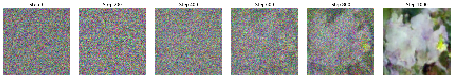
return x,sample_transitionsFinally, we have the Reverse Process. This is where the magic happens. We start with a block of pure, random Gaussian noise and slowly “chip away” at it using our trained model. At each step, the model predicts the noise, we use the math we derived earlier to calculate the “de-noised” mean ($\mu_\theta$), and then we add back a tiny bit of random variance. This randomness is crucial—it’s what allows the model to generate a different, unique flower every time even if you started with similar noise.
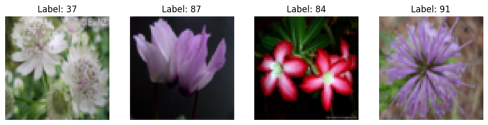
Results
I trained it for 100 epochs on a RTX 3060 laptop GPU and got a 97% loss reduction. The following are some results generated by unconditional sampling using the trained model: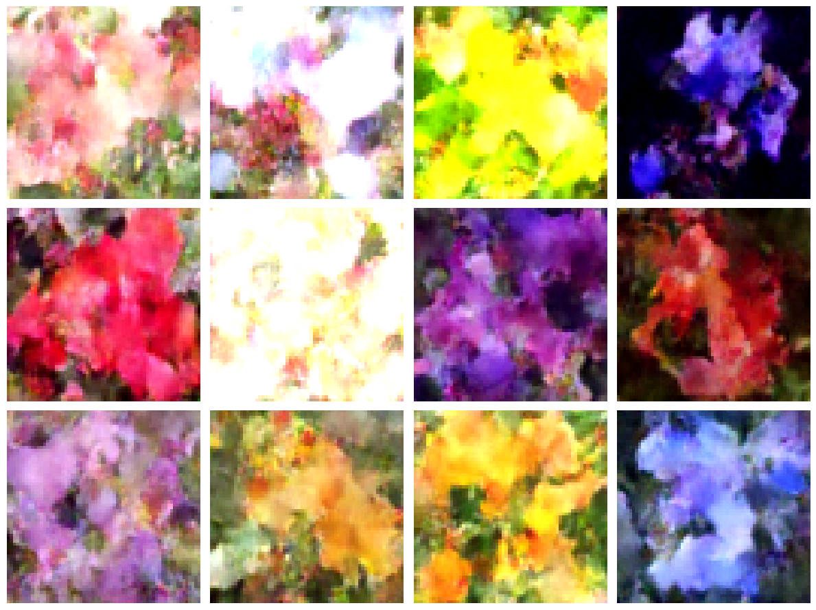
You can access the full notebook with the code here.
Let me know in the comments if any portion needs to be elaborated further. I wanted to discuss conditional generation too but I did not want to drag it further. I shall try to take it up in another blog. I also plan to write another one where we discuss the maths in more detail, deriving the expressions from first principles.
Thanks for reading :)
Resources
- DDPM: Denoising Diffusion Probabilistic Models
- Simplest Implementation of Diffusion Models | Emilio’s Blog
- Diffusion Models - The AI Summer
- Lecture Notes on Diffusion Models
- A great course on Generative Diffusion and Flow Models - YouTube
Comments
Join the discussion via GitHub.